Truncated Backprop-Through-Time (TBPTT) via tvboptim

Why the exact FC-loss gradient breaks past the chaos onset, and how a single integration.differentiation window fixes it. The adiabatic bifurcation envelope, the diagnostics swept over the global coupling \(G\) (loss, autodiff gradient, finite-difference ground truth, top Lyapunov exponent) and both optimization legs all derive from one experiment YAML via exp.run; only the plotting is hand-written. The figures reproduce the original tvboptim TBPTT.qmd workflow through the tvbo declarative pipeline.

import os

# Sweep parallelism. The motivation sweep's per-point reverse-mode AD diagnostic keeps the
# whole 60 s forward trajectory on tape, so ONE point already peaks near ~13 GB; each extra
# parallel device multiplies that. Default to sequential (1) so the page builds within a
# ~32 GB machine — the result is identical, only slower. Raise TVBO_XLA_DEVICE_COUNT (the
# reference uses 4) on a larger-RAM/GPU host to parallelise the sweep.
device_count = os.environ.get("TVBO_XLA_DEVICE_COUNT", "1")
N_PMAP = int(device_count)  # sweep parallelism = device count
os.environ["XLA_FLAGS"] = f"--xla_force_host_platform_device_count={device_count}"

import jax

jax.config.update("jax_enable_x64", True)

from tvbo import SimulationExperiment
from tvbo.datamodel.schema import Differentiation

exp = SimulationExperiment.from_db("TBPTT_JansenRit_FC_Optimization")

# The YAML already carries the reference production settings (60 s FC rollout, 20 s
# warm-up, 25-sample BOLD skip, 100 Adam steps, 80-point G sweep) — identical to the
# original tvboptim TBPTT.qmd. FC is a long-time covariance, so a stable loss landscape
# and gradient need the long rollout; trimming it (as an earlier draft did) corrupts the
# FC and the descent diverges. We keep the reference durations and cache the result. This
# is a heavy, one-time build (execute: cache).

# TBPTT leg: the YAML declares differentiation = {truncation_window: 100, mode: reverse},
# so this run uses Heun(grad_horizon=100) + reverse-mode == truncated BPTT. It also
# computes the adiabatic bifurcation scan and the motivation sweep (diagnostics vs G).
tbptt = exp.run("tvboptim", n_pmap=N_PMAP)

# Full-AD leg: identical YAML, forward-mode, no truncation window (forward-mode AD
# equals full reverse-mode BPTT for the scalar G — the exact, untruncated gradient).
exp.integration.differentiation = Differentiation(mode="forward")
ad = exp.run("tvboptim", mode="optimization")

INFO [tvbo.run] STEP 1: Running simulation...
INFO [tvbo.run]   Simulation period: 60000.0 ms, dt: 1.0 ms
INFO [tvbo.run]   Transient period: 20000.0 ms
INFO [tvbo.run]   Simulation complete.
INFO [tvbo.run] STEP 2: Running explorations...
INFO [tvbo.run]   > G_sweep
INFO [tvbo.run]   grid batch 3/80 (3%)
INFO [tvbo.run]   grid batch 6/80 (7%)
INFO [tvbo.run]   grid batch 9/80 (11%)
INFO [tvbo.run]   grid batch 12/80 (15%)
INFO [tvbo.run]   grid batch 15/80 (18%)
INFO [tvbo.run]   grid batch 18/80 (22%)
INFO [tvbo.run]   grid batch 21/80 (26%)
INFO [tvbo.run]   grid batch 24/80 (30%)
INFO [tvbo.run]   grid batch 27/80 (33%)
INFO [tvbo.run]   grid batch 30/80 (37%)
INFO [tvbo.run]   grid batch 33/80 (41%)
INFO [tvbo.run]   grid batch 36/80 (45%)
INFO [tvbo.run]   grid batch 39/80 (48%)
INFO [tvbo.run]   grid batch 42/80 (52%)
INFO [tvbo.run]   grid batch 45/80 (56%)
INFO [tvbo.run]   grid batch 48/80 (60%)
INFO [tvbo.run]   grid batch 51/80 (63%)
INFO [tvbo.run]   grid batch 54/80 (67%)
INFO [tvbo.run]   grid batch 57/80 (71%)
INFO [tvbo.run]   grid batch 60/80 (75%)
INFO [tvbo.run]   grid batch 63/80 (78%)
INFO [tvbo.run]   grid batch 66/80 (82%)
INFO [tvbo.run]   grid batch 69/80 (86%)
INFO [tvbo.run]   grid batch 72/80 (90%)
INFO [tvbo.run]   grid batch 75/80 (93%)
INFO [tvbo.run]   grid batch 78/80 (97%)
INFO [tvbo.run]   grid batch 80/80 (100%)
INFO [tvbo.run]   > motivation_sweep
INFO [tvbo.run]   grid batch 3/80 (3%)
INFO [tvbo.run]   grid batch 6/80 (7%)
INFO [tvbo.run]   grid batch 9/80 (11%)
INFO [tvbo.run]   grid batch 12/80 (15%)
INFO [tvbo.run]   grid batch 15/80 (18%)
INFO [tvbo.run]   grid batch 18/80 (22%)
INFO [tvbo.run]   grid batch 21/80 (26%)
INFO [tvbo.run]   grid batch 24/80 (30%)
INFO [tvbo.run]   grid batch 27/80 (33%)
INFO [tvbo.run]   grid batch 30/80 (37%)
INFO [tvbo.run]   grid batch 33/80 (41%)
INFO [tvbo.run]   grid batch 36/80 (45%)
INFO [tvbo.run]   grid batch 39/80 (48%)
INFO [tvbo.run]   grid batch 42/80 (52%)
INFO [tvbo.run]   grid batch 45/80 (56%)
INFO [tvbo.run]   grid batch 48/80 (60%)
INFO [tvbo.run]   grid batch 51/80 (63%)
INFO [tvbo.run]   grid batch 54/80 (67%)
INFO [tvbo.run]   grid batch 57/80 (71%)
INFO [tvbo.run]   grid batch 60/80 (75%)
INFO [tvbo.run]   grid batch 63/80 (78%)
INFO [tvbo.run]   grid batch 66/80 (82%)
INFO [tvbo.run]   grid batch 69/80 (86%)
INFO [tvbo.run]   grid batch 72/80 (90%)
INFO [tvbo.run]   grid batch 75/80 (93%)
INFO [tvbo.run]   grid batch 78/80 (97%)
INFO [tvbo.run]   grid batch 80/80 (100%)
INFO [tvbo.run]   > psp_bifurcation
INFO [tvbo.run]   psp_bifurcation 4/120 (3%)
INFO [tvbo.run]   psp_bifurcation 8/120 (6%)
INFO [tvbo.run]   psp_bifurcation 12/120 (10%)
INFO [tvbo.run]   psp_bifurcation 16/120 (13%)
INFO [tvbo.run]   psp_bifurcation 20/120 (16%)
INFO [tvbo.run]   psp_bifurcation 24/120 (20%)
INFO [tvbo.run]   psp_bifurcation 28/120 (23%)
INFO [tvbo.run]   psp_bifurcation 32/120 (26%)
INFO [tvbo.run]   psp_bifurcation 36/120 (30%)
INFO [tvbo.run]   psp_bifurcation 40/120 (33%)
INFO [tvbo.run]   psp_bifurcation 44/120 (36%)
INFO [tvbo.run]   psp_bifurcation 48/120 (40%)
INFO [tvbo.run]   psp_bifurcation 52/120 (43%)
INFO [tvbo.run]   psp_bifurcation 56/120 (46%)
INFO [tvbo.run]   psp_bifurcation 60/120 (50%)
INFO [tvbo.run]   psp_bifurcation 64/120 (53%)
INFO [tvbo.run]   psp_bifurcation 68/120 (56%)
INFO [tvbo.run]   psp_bifurcation 72/120 (60%)
INFO [tvbo.run]   psp_bifurcation 76/120 (63%)
INFO [tvbo.run]   psp_bifurcation 80/120 (66%)
INFO [tvbo.run]   psp_bifurcation 84/120 (70%)
INFO [tvbo.run]   psp_bifurcation 88/120 (73%)
INFO [tvbo.run]   psp_bifurcation 92/120 (76%)
INFO [tvbo.run]   psp_bifurcation 96/120 (80%)
INFO [tvbo.run]   psp_bifurcation 100/120 (83%)
INFO [tvbo.run]   psp_bifurcation 104/120 (86%)
INFO [tvbo.run]   psp_bifurcation 108/120 (90%)
INFO [tvbo.run]   psp_bifurcation 112/120 (93%)
INFO [tvbo.run]   psp_bifurcation 116/120 (96%)
INFO [tvbo.run]   psp_bifurcation 120/120 (100%)
INFO [tvbo.run]   Explorations complete.
INFO [tvbo.run] STEP 4: Running optimization...
INFO [tvbo.run]   step 0/100: loss=0.33267
INFO [tvbo.run]   step 10/100: loss=0.241011
INFO [tvbo.run]   step 20/100: loss=0.296244
INFO [tvbo.run]   step 30/100: loss=0.245115
INFO [tvbo.run]   step 40/100: loss=0.244604
INFO [tvbo.run]   step 50/100: loss=0.241365
INFO [tvbo.run]   step 60/100: loss=0.244974
INFO [tvbo.run]   step 70/100: loss=0.252336
INFO [tvbo.run]   step 80/100: loss=0.252275
INFO [tvbo.run]   step 90/100: loss=0.254923
INFO [tvbo.run]   Optimization complete.
INFO [tvbo.run] Experiment complete.
INFO [tvbo.run] STEP 1: Running simulation...
INFO [tvbo.run]   Simulation period: 60000.0 ms, dt: 1.0 ms
INFO [tvbo.run]   Transient period: 20000.0 ms
INFO [tvbo.run]   Simulation complete.
INFO [tvbo.run] STEP 4: Running optimization...
INFO [tvbo.run]   step 0/100: loss=0.33267
INFO [tvbo.run]   step 10/100: loss=0.331154
INFO [tvbo.run]   step 20/100: loss=0.330666
INFO [tvbo.run]   step 30/100: loss=0.33165
INFO [tvbo.run]   step 40/100: loss=0.331647
INFO [tvbo.run]   step 50/100: loss=0.315586
INFO [tvbo.run]   step 60/100: loss=0.325888
INFO [tvbo.run]   step 70/100: loss=0.331115
INFO [tvbo.run]   step 80/100: loss=0.332159
INFO [tvbo.run]   step 90/100: loss=0.332273
INFO [tvbo.run]   Optimization complete.
INFO [tvbo.run] Experiment complete.

The problem: the exact gradient breaks at the bifurcation

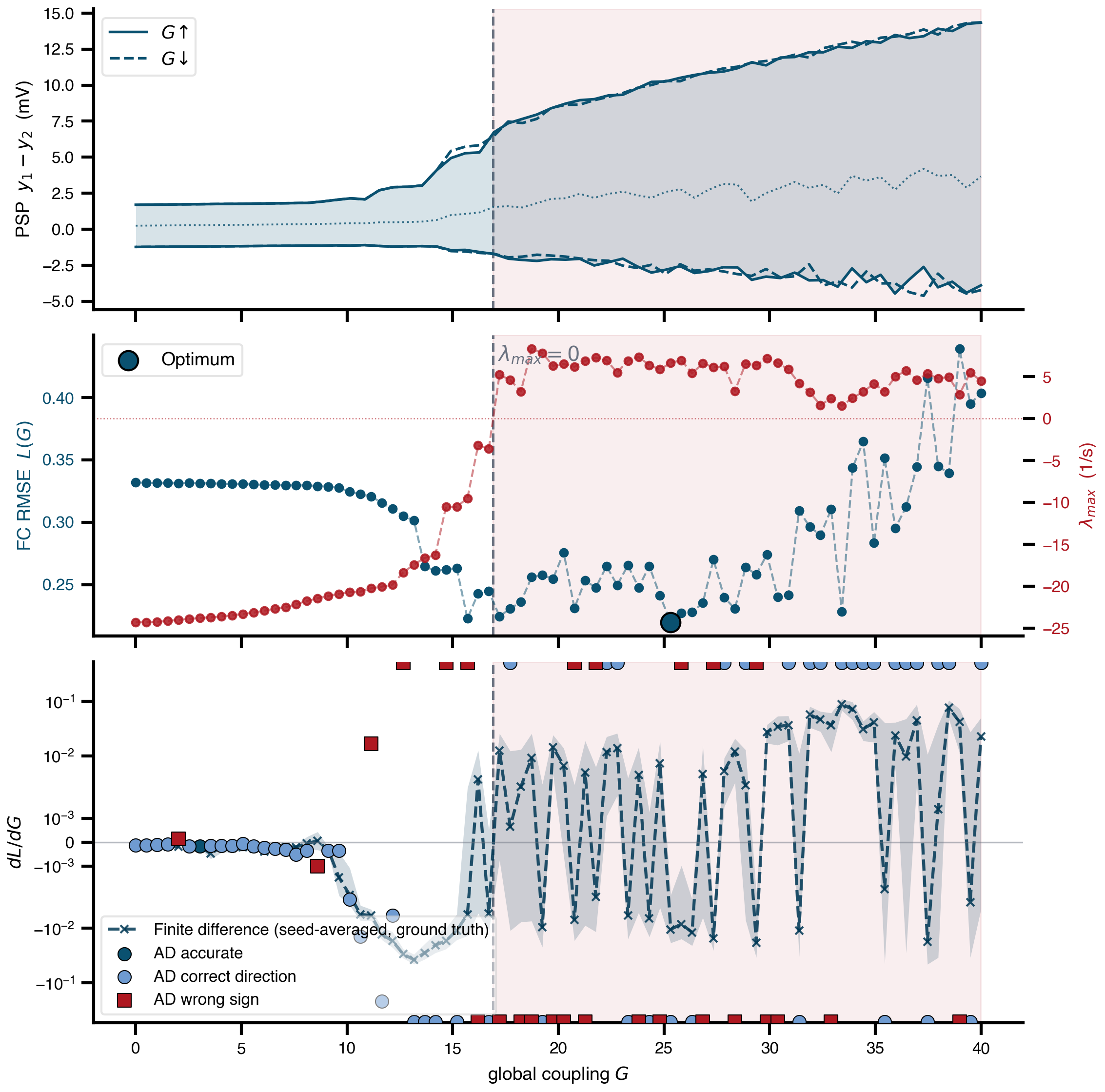
The loss is the RMSE between the simulated FC and the empirical target. Swept over \(G\), the network runs from a quiescent fixed point, through synchronized oscillation, into chaos, where the exact reverse-mode gradient of a long-rollout FC loss amplifies without bound and flips sign. The adiabatic scan reads that transition straight off the dynamics; the Lyapunov exponent flags the same onset.

Show plotting code

def categorize(ad, fd, eps=0.01):
    ad, fd = np.asarray(ad, float), np.asarray(fd, float)
    ad_ok = ~(np.isnan(ad) | np.isinf(ad))
    rel = np.where(np.abs(fd) > 1e-12, np.abs(ad - fd) / np.abs(fd), np.inf)
    same_sign = np.sign(np.where(ad_ok, ad, 0.0)) == np.sign(fd)
    accurate = ad_ok & (rel < eps)
    correct = ad_ok & same_sign & ~accurate
    wrong = ad_ok & ~same_sign
    unstable = ~ad_ok
    return accurate, correct, wrong, unstable


fig, (ax_bif, ax_top, ax_bot) = plt.subplots(
    3, 1, figsize=(8.2, 9.0), sharex=True,
    gridspec_kw={"height_ratios": [1.0, 1.0, 1.2], "hspace": 0.08},
)


def chaos_band(ax):
    """Shade the chaotic band and mark the lambda_max=0 boundary."""
    if G_CRIT is not None:
        ax.axvspan(G_CRIT, G.max(), color=WARN, alpha=0.07, zorder=0)
        ax.axvline(G_CRIT, color=ROAD, ls="--", lw=1.2, zorder=0)


# ---- top: adiabatic bifurcation envelope (mean dynamics vs G) ----
up, dn = slice(0, n_up), slice(n_up, None)
chaos_band(ax_bif)
ax_bif.fill_between(pp[up], psp_lo[up], psp_hi[up], color=ACCENT, alpha=0.16, lw=0, zorder=1)
ax_bif.plot(pp[up], psp_hi[up], color=ACCENT, lw=1.3, zorder=2, label=r"$G\!\uparrow$")
ax_bif.plot(pp[up], psp_lo[up], color=ACCENT, lw=1.3, zorder=2)
ax_bif.plot(pp[up], psp_mean[up], color=ACCENT, lw=0.9, ls=":", alpha=0.8, zorder=2)
ax_bif.plot(pp[dn], psp_hi[dn], color=ACCENT, lw=1.3, ls="--", zorder=3, label=r"$G\!\downarrow$")
ax_bif.plot(pp[dn], psp_lo[dn], color=ACCENT, lw=1.3, ls="--", zorder=3)
ax_bif.set_ylabel(r"PSP  $y_1 - y_2$  (mV)")
ax_bif.legend(loc="upper left", fontsize=9, framealpha=0.5)

# ---- middle: loss + Lyapunov exponent (chaos onset) ----
lam_ax = ax_top.twinx()
chaos_band(ax_top)
ax_top.plot(G, loss_G, "--", color=ACCENT, lw=1.0, alpha=0.5, zorder=2)
ax_top.scatter(G, loss_G, color=ACCENT, s=14, zorder=3)
kbest = int(np.nanargmin(loss_G))
ax_top.scatter([G[kbest]], [loss_G[kbest]], color=ACCENT, s=90, edgecolor="black",
               linewidth=1.0, zorder=4, label="Optimum")
ax_top.set_ylabel("FC RMSE  $L(G)$", color=ACCENT)
ax_top.tick_params(axis="y", labelcolor=ACCENT)
ax_top.legend(loc="upper left", fontsize=9, framealpha=0.5)
lam_ax.plot(G, lyap_G, "--", color=WARN, lw=1.0, alpha=0.5, zorder=2)
lam_ax.scatter(G, lyap_G, color=WARN, s=14, alpha=0.85, zorder=3)
lam_ax.axhline(0.0, color=WARN, lw=0.6, ls=":", alpha=0.6)
lam_ax.set_ylabel(r"$\lambda_{max}$  (1/s)", color=WARN)
lam_ax.tick_params(axis="y", labelcolor=WARN)
if G_CRIT is not None:
    lam_ax.text(G_CRIT, 0.97, r" $\lambda_{max}=0$", color=ROAD, va="top",
                ha="left", transform=lam_ax.get_xaxis_transform(), fontsize=10)

# ---- bottom: AD gradient vs FD ground truth (adaptive symlog) ----
fd_abs = np.abs(fd_G[np.isfinite(fd_G)])
cap = float(6.0 * np.nanmax(fd_abs)) if fd_abs.size else 1.0
lin = float(max(0.3 * np.nanmedian(fd_abs), 1e-9)) if fd_abs.size else 1e-3
chaos_band(ax_bot)
ax_bot.fill_between(G, fd_G - fd_sem, fd_G + fd_sem, color=INK, alpha=0.18, lw=0)
ax_bot.plot(G, fd_G, "x--", color=INK, alpha=0.85, label="Finite difference (seed-averaged, ground truth)")
acc, cor, wro, uns = categorize(ad_G, fd_G)
ad_disp = np.clip(np.asarray(ad_G, float), -cap * 0.96, cap * 0.96)
for mask, color, marker, label in [
    (acc, ACCENT, "o", "AD accurate"),
    (cor, "#6f9bd1", "o", "AD correct direction"),
    (wro, WARN, "s", "AD wrong sign"),
    (uns, WARN, "X", "AD unstable (NaN/Inf)"),
]:
    if np.any(mask):
        y = np.where(uns, 0.0, ad_disp)[mask] if label.endswith("(NaN/Inf)") else ad_disp[mask]
        ax_bot.scatter(G[mask], y, color=color, marker=marker, s=42,
                       edgecolor="black", linewidth=0.5, zorder=3, label=label)
ax_bot.set_yscale("symlog", linthresh=lin, linscale=0.8)
ax_bot.set_ylim(-cap, cap)
ax_bot.axhline(0.0, color=ROAD, lw=0.8, alpha=0.5)
ax_bot.set_xlabel(r"global coupling $G$")
ax_bot.set_ylabel(r"$dL/dG$")
ax_bot.legend(loc="lower left", fontsize=8, framealpha=0.5)
plt.tight_layout()
plt.show()

/var/folders/ym/9kw1g21j1nd7kwfn8c0z3st40000gn/T/ipykernel_28211/1267832490.py:83: UserWarning: This figure includes Axes that are not compatible with tight_layout, so results might be incorrect.
  plt.tight_layout()

Figure 1: **The exact FC-loss gradient breaks at the chaos onset.** All three panels share the global-coupling axis \(G\), with the chaotic band (\(\lambda_{max}>0\)) shaded red. Top: the adiabatic bifurcation envelope of the pyramidal PSP \(y_1 - y_2\) (per-node temporal min/max averaged across the network; dotted = mean), swept up (\(G\!\uparrow\), solid) and back down (\(G\!\downarrow\), dashed) — flat at the fixed point, opening at the limit cycle, broad in chaos, with the branches revealing any hysteresis. Middle: the FC-RMSE loss \(L(G)\) (blue, left) and the top Lyapunov exponent \(\lambda_{max}\) (red, right), which crosses zero at the bifurcation; the loss optimum (blue dot) sits just below it. Bottom: the gradient \(dL/dG\) — the seed-averaged finite-difference gradient (line + \(\pm\)SEM band) is the ground truth; the autodiff gradient (markers) is coloured by how it compares (accurate within 1%, correct direction, wrong sign, unstable). AD tracks FD until \(G\) crosses \(\lambda_{max}=0\), then flips sign and blows up.

The fix: truncating the gradient horizon

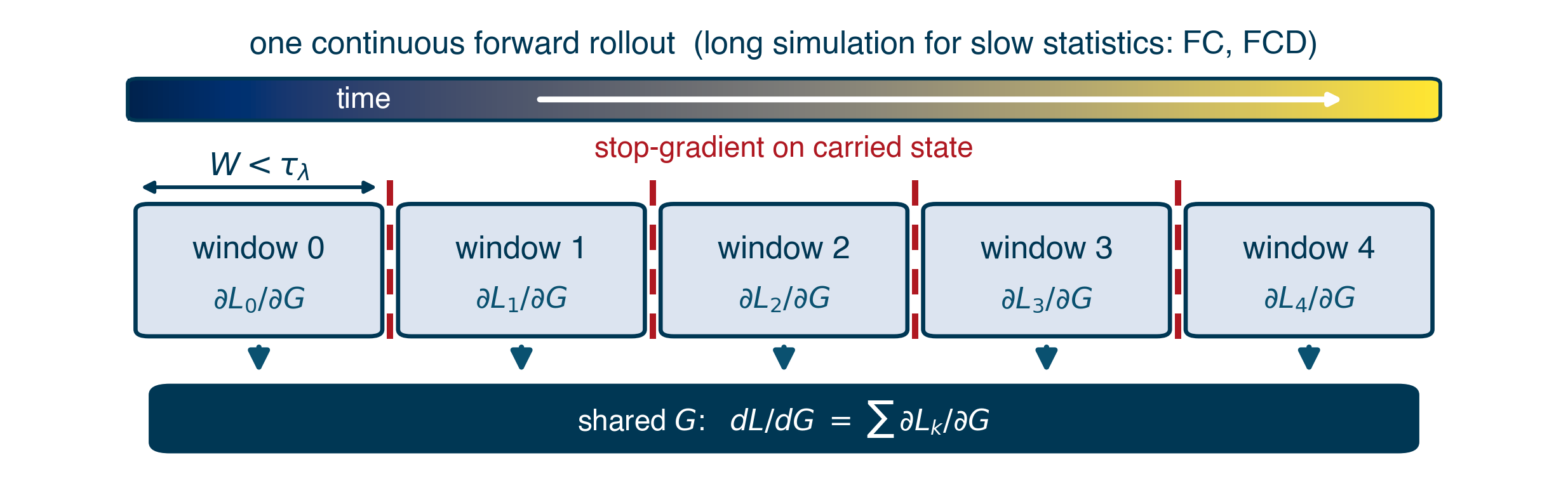
Truncated backprop-through-time keeps the long forward rollout but pulls the gradient back only through a fixed window of \(W =\) grad_horizon steps (integration.differentiation.truncation_window). Every window is differentiated and contributes its local \(\partial L_k/\partial G\); the carried state gradient is severed at each window boundary with stop_gradient, so the \(\exp(T\,\lambda_{max})\) blow-up is cut off at \(W\), while the shared parameter gradient survives as the sum over windows.

Show diagram code

N_WIN, W = 5, 1.0
BOX_Y0, BOX_H = 0.0, 0.95
TOP_Y0, TOP_H = 1.55, 0.30

fig, ax = plt.subplots(figsize=(8.4, 2.7))
ax.imshow(np.linspace(0, 1, 256)[None, :], extent=(0, N_WIN * W, TOP_Y0, TOP_Y0 + TOP_H),
          aspect="auto", cmap="cividis", zorder=1)
ax.add_patch(FancyBboxPatch((0, TOP_Y0), N_WIN * W, TOP_H,
             boxstyle="round,pad=0,rounding_size=0.04", fill=False, edgecolor=INK, lw=1.4, zorder=2))
ax.text(N_WIN * W / 2, TOP_Y0 + TOP_H + 0.14,
        "one continuous forward rollout  (long simulation for slow statistics: FC, FCD)",
        ha="center", va="bottom", fontsize=12, color=INK)
ax.annotate("", xy=(N_WIN * W - 0.35, TOP_Y0 + TOP_H / 2), xytext=(1.55, TOP_Y0 + TOP_H / 2),
            arrowprops=dict(arrowstyle="-|>", color="white", lw=2.2))
ax.text(0.9, TOP_Y0 + TOP_H / 2, "time", ha="center", va="center", fontsize=11, color="white", style="italic")
for k in range(N_WIN):
    x0 = k * W
    ax.add_patch(FancyBboxPatch((x0 + 0.03, BOX_Y0), W - 0.06, BOX_H,
                 boxstyle="round,pad=0,rounding_size=0.05", facecolor=WIN, edgecolor=INK, lw=1.6, zorder=3))
    ax.text(x0 + W / 2, BOX_Y0 + BOX_H * 0.66, f"window {k}", ha="center", va="center", fontsize=12, color=INK)
    ax.text(x0 + W / 2, BOX_Y0 + BOX_H * 0.28, r"$\partial L_{%d}/\partial G$" % k,
            ha="center", va="center", fontsize=11, color=ACCENT)
    ax.add_patch(FancyArrowPatch((x0 + W / 2, BOX_Y0 - 0.04), (x0 + W / 2, BOX_Y0 - 0.30),
                 arrowstyle="-|>", mutation_scale=16, color=ACCENT, lw=2.0, zorder=4))
    if k > 0:
        ax.plot([x0, x0], [BOX_Y0 - 0.02, BOX_Y0 + BOX_H + 0.22], color=WARN, lw=2.4, ls=(0, (4, 3)), zorder=5)
ax.text(N_WIN * W / 2, BOX_Y0 + BOX_H + 0.30, "stop-gradient on carried state",
        ha="center", va="bottom", fontsize=11, color=WARN, weight="bold")
ax.annotate("", xy=(W - 0.03, BOX_Y0 + BOX_H + 0.12), xytext=(0.03, BOX_Y0 + BOX_H + 0.12),
            arrowprops=dict(arrowstyle="<|-|>", color=INK, lw=1.4))
ax.text(W / 2, BOX_Y0 + BOX_H + 0.16, r"$W < \tau_\lambda$", ha="center", va="bottom", fontsize=12, color=INK)
sum_top, box_h, box_w = BOX_Y0 - 0.36, 0.46, 4.8
ax.add_patch(FancyBboxPatch((N_WIN * W / 2 - box_w / 2, sum_top - box_h), box_w, box_h,
             boxstyle="round,pad=0.02,rounding_size=0.08", facecolor=INK, edgecolor="none", zorder=4))
ax.text(N_WIN * W / 2, sum_top - box_h / 2, r"shared $G$:   $dL/dG \;=\; \sum\, \partial L_k/\partial G$",
        ha="center", va="center", fontsize=11, color="white", zorder=5)
ax.set_xlim(-0.45, N_WIN * W + 0.45)
ax.set_ylim(sum_top - box_h - 0.15, TOP_Y0 + TOP_H + 0.5)
ax.axis("off")
plt.tight_layout()
plt.show()

Figure 2: **How `grad_horizon` tiles the rollout.** One continuous forward pass (top strip, colour = time) is split into windows of \(W\) steps. Every window is differentiated and contributes its local \(\partial L_k/\partial G\), but the carried-state gradient is cut at every boundary (red dashed). The shared \(G\) is closed over by all windows, so its gradient is the sum of the per-window contributions; the window is kept below the chaotic memory horizon, \(W < \tau_\lambda\).

The payoff: optimizing \(G\) with and without truncation

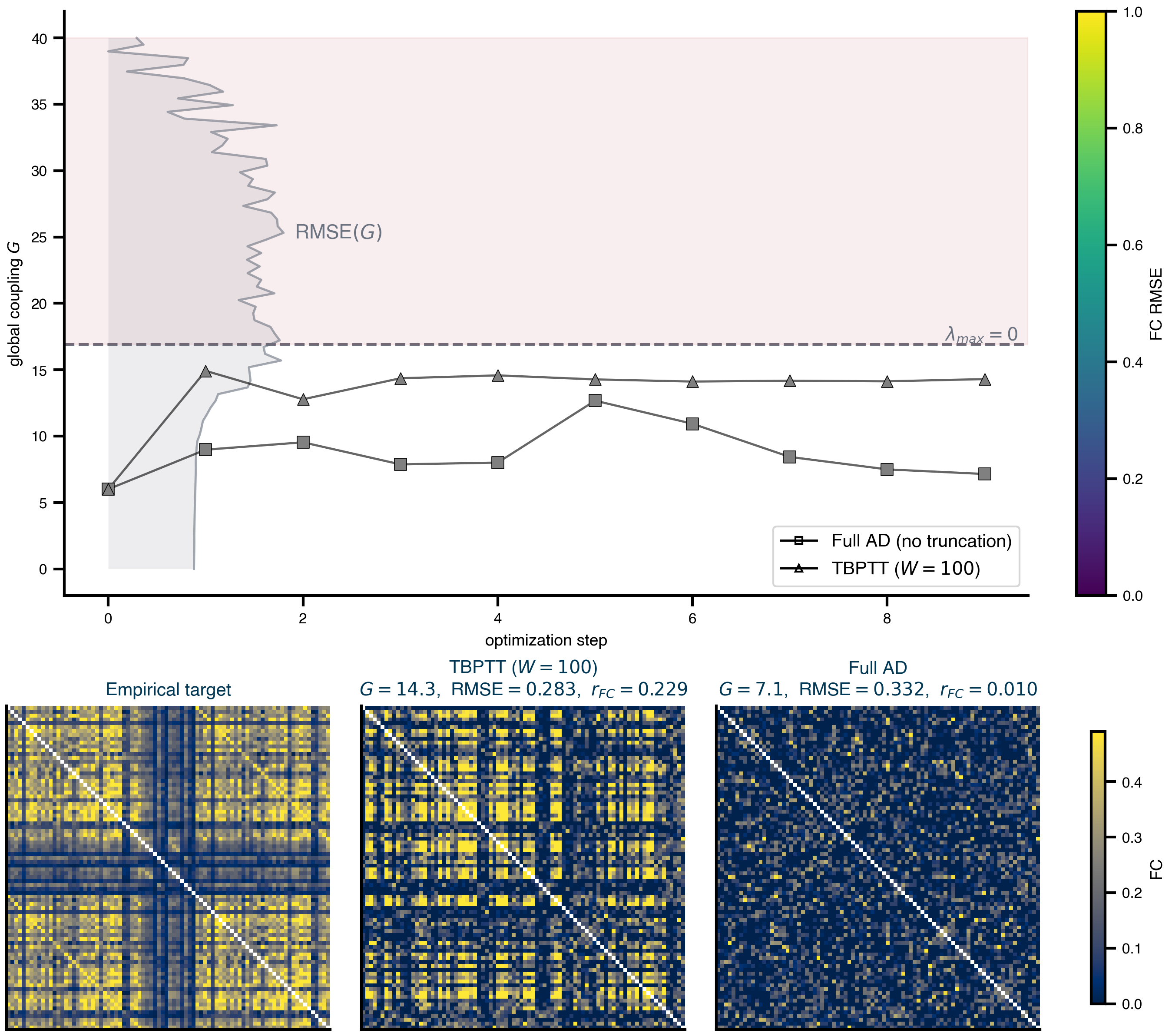
Both legs fit \(G\) to the empirical FC from the same sub-critical start with the same optimizer, differing only in how the gradient is obtained: full AD (the exact, untruncated gradient) versus TBPTT (grad_horizon window). The full-AD run is driven by the unstable gradient into the chaotic band; the TBPTT run descends on a stable, short-horizon gradient and settles near the RMSE optimum on the stable side.

Show plotting code

fig = plt.figure(figsize=(9.0, 8.0), layout="constrained")
gs = fig.add_gridspec(2, 1, height_ratios=[1.5, 1.0])
ax = fig.add_subplot(gs[0])
gs_fc = gs[1].subgridspec(1, 3, wspace=0.08)
fc_axes = [fig.add_subplot(gs_fc[0, j]) for j in range(3)]

g_top = max(np.nanmax(ad_G_traj), np.nanmax(tb_G))
if G_CRIT is not None:
    ax.axhline(G_CRIT, color=ROAD, ls="--", lw=1.5, zorder=0)
    ax.axhspan(G_CRIT, max(g_top * 1.05, G.max()), color=WARN, alpha=0.07, zorder=0)
    ax.text(0.99, G_CRIT, r"$\lambda_{max}=0$ ", color=ROAD, va="bottom", ha="right",
            transform=ax.get_yaxis_transform(), fontsize=10)

# sideways RMSE(G) reference profile (bulges right at the minimum = optimum)
MAX_STEPS = max(len(tb_step), len(ad_step))
PROFILE_X0, PROFILE_W = 0.0, 0.18 * MAX_STEPS
emin, emax = float(np.nanmin(loss_G)), float(np.nanmax(loss_G))
if emax > emin:
    xprof = PROFILE_X0 + PROFILE_W * (emax - loss_G) / (emax - emin)
    order = np.argsort(G)
    ax.fill_betweenx(G[order], PROFILE_X0, xprof[order], color=ROAD, alpha=0.12, lw=0, zorder=0)
    ax.plot(xprof[order], G[order], color=ROAD, lw=1.2, alpha=0.6, zorder=1)
    kbest = int(np.nanargmin(loss_G))
    ax.annotate(r"RMSE$(G)$", xy=(xprof[kbest], G[kbest]), xytext=(6, 0),
                textcoords="offset points", color=ROAD, fontsize=11, va="center")

# trajectories, coloured by FC-RMSE on a shared scale
_rmses = [r for r in (tb_rmse, ad_rmse) if r is not None]
if _rmses:
    allr = np.concatenate(_rmses)
    vmin, vmax = float(np.nanmin(allr)), float(np.nanmax(allr))
else:
    vmin, vmax = 0.0, 1.0
runs_plot = [
    (ad_step, ad_G_traj, ad_rmse, "s", "Full AD (no truncation)"),
    (tb_step, tb_G, tb_rmse, "^", f"TBPTT ($W=100$)"),
]
sc = None
for steps, Gtraj, err, marker, _ in runs_plot:
    ax.plot(steps, Gtraj, color="black", lw=1.2, alpha=0.6, zorder=2)
    c = err if err is not None else "gray"
    sc = ax.scatter(steps, Gtraj, c=c, cmap="cividis_r", vmin=vmin, vmax=vmax,
                    marker=marker, s=42, edgecolor="black", linewidth=0.4, zorder=3)
ax.set_xlabel("optimization step")
ax.set_ylabel(r"global coupling $G$")
if sc is not None:
    fig.colorbar(sc, ax=ax, label="FC RMSE")
handles = [Line2D([0], [0], color="black", marker=m, lw=1.2, markerfacecolor="none",
                  markeredgecolor="black", label=lab) for _, _, _, m, lab in runs_plot]
ax.legend(handles=handles, loc="best", fontsize=10)

# ---- bottom: simulated FC at each run's optimum vs the empirical target ----
panels = [
    ("Empirical target", fc_target, None, None),
    (f"TBPTT ($W=100$)", fc_tbptt, tb_G_final, tbptt),
    ("Full AD", fc_ad, ad_G_final, ad),
]
mats = np.array([p[1] for p in panels])
offdiag = ~np.eye(mats.shape[1], dtype=bool)
vmax_fc = float(np.nanpercentile(mats[:, offdiag], 95))
im = None
for fa, (title, mat, Gval, _res) in zip(fc_axes, panels):
    m = np.array(mat, float)
    np.fill_diagonal(m, np.nan)
    im = fa.imshow(m, cmap="cividis", vmin=0.0, vmax=vmax_fc, aspect="equal", interpolation="none")
    fa.set_xticks([])
    fa.set_yticks([])
    if Gval is None:
        sub = title
    else:
        rmse_v = float(np.sqrt(np.nanmean((np.array(mat) - np.array(fc_target)) ** 2)))
        a, b = np.array(mat)[offdiag], np.array(fc_target)[offdiag]
        r_v = float(np.corrcoef(a, b)[0, 1])
        sub = f"{title}\n$G={Gval:.1f}$,  RMSE$={rmse_v:.3f}$,  $r_{{FC}}={r_v:.3f}$"
    fa.set_title(sub, fontsize=10, color=INK)
fig.colorbar(im, ax=fc_axes, label="FC", shrink=0.8)
plt.show()

/var/folders/ym/9kw1g21j1nd7kwfn8c0z3st40000gn/T/ipykernel_28211/3202694252.py:42: UserWarning: No data for colormapping provided via 'c'. Parameters 'cmap', 'vmin', 'vmax' will be ignored
  sc = ax.scatter(steps, Gtraj, c=c, cmap="cividis_r", vmin=vmin, vmax=vmax,

Figure 3: **Optimizing \(G\) to fit FC, with and without truncation.** Top: each trajectory is one run; the y-axis is \(G\) at each optimization step, points coloured by the FC-RMSE they reached. The dashed line is the \(\lambda_{max}=0\) boundary, the red band the chaotic regime, and the grey curve the \(RMSE(G)\) profile from the sweep (bulging right at the optimum). Full AD is driven into the chaotic band; TBPTT settles near the optimum on the stable side. Bottom: the simulated FC at each run’s optimized \(G\) beside the empirical target — the TBPTT fit reproduces the target structure, the full-AD run does not.

One experiment, three views

The adiabatic envelope, the diagnostics sweep, and both descent legs all come from the same TBPTT_JansenRit_FC_Optimization YAML. The bifurcation scan is a declarative strategy: adiabatic_scan exploration, the diagnostics are analysis observations recorded over a G sweep, and the truncation window is a single integration.differentiation.truncation_window. Only the plotting above is hand-written.