FitzHugh-Nagumo Brain Synchronization

Directed weighted coupling on a 90-region brain atlas

Replicates the NetworkDynamics.jl Directed and Weighted Graphs tutorial — FitzHugh-Nagumo oscillators on a 90-region AAL brain connectivity derived from DTI (Tzourio-Mazoyer et al., 2002). The structural connectivity matrix Norm_G_DTI.txt provides directed, weighted edges.

YAML Specification

# =============================================================================
# FitzHugh-Nagumo on a Directed Weighted Brain Network
# =============================================================================
# Source: https://juliadynamics.github.io/NetworkDynamics.jl/stable/generated/directed_and_weighted_graphs/
#
# FitzHugh-Nagumo relaxation oscillators coupled via electrical gap junctions
# on a directed, weighted 90-region brain connectivity (AAL atlas).
# =============================================================================

id: 102
label: "FitzHugh-Nagumo Brain Synchronization"
description: >
    Neurodynamic model of synchronization: FitzHugh-Nagumo oscillators
    coupled through weighted, directed electrical gap junctions on a
    90-region brain atlas (AAL, Tzourio-Mazoyer et al., 2002).
    Recreates the NetworkDynamics.jl Directed and Weighted Graphs tutorial.
references:
    - "https://juliadynamics.github.io/NetworkDynamics.jl/stable/generated/directed_and_weighted_graphs/"
    - "FitzHugh, R. (1961). Impulses and physiological states in theoretical models of nerve membrane. Biophysical Journal, 1(6), 445-466."
    - "Nagumo, J., Arimoto, S., & Yoshizawa, S. (1962). An active pulse transmission line simulating nerve axon. Proceedings of the IRE, 50(10), 2061-2070."
    - "Tzourio-Mazoyer, N., et al. (2002). Automated anatomical labeling of activations in SPM. Neuroimage, 15(1), 273-289."

# -- Local Dynamics ------------------------------------------------------------
dynamics:
    name: FitzHughNagumo
    label: "FitzHugh-Nagumo oscillator"
    description: >
        Two-variable relaxation oscillator. u is the fast excitatory
        variable (membrane potential analogue), v is the slow inhibitory
        recovery variable.
        eps du/dt = u - u^3/3 - v + esum;  dv/dt = (u + a) eps
    system_type: continuous
    autonomous: true
    has_reference: "FitzHugh1961"
    parameters:
        a:
            label: "Control parameter"
            symbol: "a"
            value: 0.5
            unit: "1"
            description: "Excitability threshold; determines oscillatory vs excitable regime"
        epsilon:
            label: "Time-scale separation"
            symbol: "epsilon"
            value: 0.05
            unit: "1"
            description: "Ratio of fast (u) to slow (v) time scales"
    coupling_terms:
        c_electrical:
            description: "Aggregated electrical gap-junction coupling (sum of incident edge outputs)"
    state_variables:
        u:
            label: "Fast excitatory variable"
            symbol: "u"
            equation:
                rhs: "u - u**3 / 3 - v + c_electrical"
                description: "du/dt = u - u^3/3 - v + sum(edges)"
            initial_value: 0.0
            distribution:
                name: Gaussian
                seed: 42
                domain: { lo: -15.0, hi: 15.0 }
                parameters:
                    mean: { name: mean, value: 0.0 }
                    std: { name: std, value: 5.0 }
            unit: "mV"
            variable_of_interest: true
            coupling_variable: true
        v:
            label: "Slow inhibitory variable"
            symbol: "v"
            equation:
                rhs: "(u - a) * epsilon"
                description: "dv/dt = (u - a) eps"
            initial_value: 0.0
            distribution:
                name: Gaussian
                seed: 42
                domain: { lo: -15.0, hi: 15.0 }
                parameters:
                    mean: { name: mean, value: 0.0 }
                    std: { name: std, value: 5.0 }
            unit: "mV"
            variable_of_interest: true

# -- Network -------------------------------------------------------------------
network:
    label: "AAL-90 directed brain network"
    description: >
        Directed, weighted structural connectivity from diffusion tensor
        imaging.  90 cortical regions from the Automated Anatomical Labeling
        (AAL) atlas (Tzourio-Mazoyer et al., 2002).  Edge weights are set
        at runtime from the Norm_G_DTI.txt matrix.
    number_of_nodes: 90
    edge_matrix_files:
        - ../Norm_G_DTI.txt
    parcellation:
        label: "AAL-90"
        atlas:
            name: "AAL"
    distance_unit: "mm"

    coupling:
        ElectricalCoupling:
            name: ElectricalCoupling
            label: "Weighted electrical gap-junction coupling"
            description: >
                Directed coupling: each edge computes w * sigma * (u_src - u_dst),
                where w is the per-edge structural weight and sigma is a global
                coupling strength parameter.
            delayed: false
            parameters:
                w:
                    label: "Edge weight"
                    symbol: "w"
                    value: 1.0
                    unit: "1"
                    description: "Structural connectivity weight (per-edge, from DTI)"
                sigma:
                    label: "Global coupling strength"
                    symbol: "sigma"
                    value: 0.5
                    unit: "1"
                    description: "Global scaling of electrical gap-junction coupling"
            pre_expression:
                rhs: "w * sigma * (x_j - x_i)"
                description: "Directed weighted diffusive coupling"

# -- Integration ---------------------------------------------------------------
integration:
    description: >
        Automatic stiffness-detecting solver: Tsit5 with fallback to TRBDF2.
        dt=0.1 over t in [0, 200].
    method: AutoTsit5
    step_size: 0.1
    duration: 200.0
    time_scale: "ms"

Model Report

FitzHugh-Nagumo Brain Synchronization

Neurodynamic model of synchronization: FitzHugh-Nagumo oscillators coupled through weighted, directed electrical gap junctions on a 90-region brain atlas (AAL, Tzourio-Mazoyer et al., 2002). Recreates the NetworkDynamics.jl Directed and Weighted Graphs tutorial.

1. Brain Network: AAL-90 directed brain network

Directed, weighted structural connectivity from diffusion tensor imaging. 90 cortical regions from the Automated Anatomical Labeling (AAL) atlas (Tzourio-Mazoyer et al., 2002). Edge weights are set at runtime from the Norm_G_DTI.txt matrix.

Parcellation: AAL-90 (AAL)
Regions: 90

Coupling: Weighted electrical gap-junction coupling

Directed coupling: each edge computes w * sigma * (u_src - u_dst), where w is the per-edge structural weight and sigma is a global coupling strength parameter.

Receives \(u\) from connected regions.

Pre-synaptic: \(c_{\text{pre}} = \sigma \cdot w \cdot \left(x_{j} - x_{i}\right)\)

Parameter	Value	Description
\(\sigma\)	0.5	Global scaling of electrical gap-junction coupling
\(w\)	1.0	Structural connectivity weight (per-edge, from DTI)

2. Local Dynamics: FitzHugh-Nagumo oscillator

Two-variable relaxation oscillator. The model comprises 2 state variables.

2.1 State Equations

\[\dot{u} = c_{\mathcal{electri}} + u - v - \frac{u^{3}}{3}\]

\[\dot{v} = \epsilon \cdot \left(u - a\right)\]

2.2 Parameters

Parameter	Value	Unit	Description
\(a\)	0.5	dimensionless	Excitability threshold; determines oscillatory vs excitable regime
\(\epsilon\)	0.05	dimensionless	Ratio of fast (u) to slow (v) time scales

3. Numerical Integration

Method: AutoTsit5
Time step: \(\Delta t = 0.1\) ms
Duration: 200.0 ms

References

https://juliadynamics.github.io/NetworkDynamics.jl/stable/generated/directed_and_weighted_graphs/
FitzHugh, R. (1961). Impulses and physiological states in theoretical models of nerve membrane. Biophysical Journal, 1(6), 445-466.
Nagumo, J., Arimoto, S., & Yoshizawa, S. (1962). An active pulse transmission line simulating nerve axon. Proceedings of the IRE, 50(10), 2061-2070.
Tzourio-Mazoyer, N., et al. (2002). Automated anatomical labeling of activations in SPM. Neuroimage, 15(1), 273-289.

Generated Julia Code

Code(exp.render_code("networkdynamics"), language='julia')

using Graphs
using NetworkDynamics

using OrdinaryDiffEqTsit5
using OrdinaryDiffEqSDIRK
using DelimitedFiles
using SimpleWeightedGraphs







function FitzHughNagumo_f!(dx, x, esum, (a, epsilon,), t)

    u, v = x

    c_electrical = esum[1]
    dx[1] = c_electrical + u - v - u .^ 3 / 3
    dx[2] = epsilon .* (u - a)
    nothing
end

vertex_FitzHughNagumo = VertexModel(;
    f = FitzHughNagumo_f!,
    g = StateMask(1:1),
    sym = [:u, :v],
    psym = [:a => 0.5, :epsilon => 0.05],
    name = :FitzHughNagumo,
)








function ElectricalCoupling_edge_g!(e_dst, v_src, v_dst, (sigma, w,), t)
    e_dst[1] = sigma .* w .* (v_src[1] - v_dst[1])
    nothing
end

edge_ElectricalCoupling = EdgeModel(;
    g = Directed(ElectricalCoupling_edge_g!),
    outsym = [:coupling],
    psym = [:sigma => 0.5, :w => 1.0],
    name = :ElectricalCoupling,
)




G = readdlm("../Norm_G_DTI.txt", ',', Float64, '\n')
g_weighted = SimpleWeightedDiGraph(G)
edge_weights = getfield.(collect(edges(g_weighted)), :weight)
g = SimpleDiGraph(g_weighted)


nw = Network(g, vertex_FitzHughNagumo, edge_ElectricalCoupling)

p = NWParameter(nw)
p.e[1:ne(g), :w] = edge_weights




s = NWState(nw)
using Random
rng = MersenneTwister(42)

for node in 1:nv(g)
    s.v[node, :u] = 0.0 .+ 5.0 .* randn(rng)
end

for node in 1:nv(g)
    s.v[node, :v] = 0.0 .+ 5.0 .* randn(rng)
end



tspan = (0.0, 200.0)
prob = ODEProblem(nw, uflat(s), tspan, pflat(p))
sol = solve(prob, AutoTsit5(TRBDF2()); saveat=0.1)

adj_matrix = Float64.(adjacency_matrix(g))

using Random: MersenneTwister
function spring_layout(g; seed=42, iterations=50, k=1.0)
    rng = MersenneTwister(seed)
    n = nv(g)
    pos = randn(rng, n, 2)
    for _ in 1:iterations
        disp = zeros(n, 2)
        for i in 1:n, j in (i+1):n
            d = pos[i, :] - pos[j, :]
            dist = max(norm(d), 0.01)
            rep = k^2 / dist
            disp[i, :] .+= d / dist * rep
            disp[j, :] .-= d / dist * rep
        end
        for e in edges(g)
            i, j = src(e), dst(e)
            d = pos[j, :] - pos[i, :]
            dist = max(norm(d), 0.01)
            att = dist^2 / k
            disp[i, :] .+= d / dist * att
            disp[j, :] .-= d / dist * att
        end
        for i in 1:n
            dl = max(norm(disp[i, :]), 0.01)
            pos[i, :] .+= disp[i, :] / dl * min(dl, 0.1)
        end
    end
    return pos
end
using LinearAlgebra: norm
node_positions = spring_layout(g)

using Plots
plot(sol; ylabel="state", xlabel="time", title="FitzHughNagumo on 90-node network")

Run & Plot

ts = exp.run(format="networkdynamics")
ts.plot()

Detected IPython. Loading juliacall extension. See https://juliapy.github.io/PythonCall.jl/stable/compat/#IPython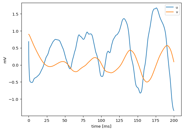

Results

Shape: (2001, 2, 90)
Time range: 0.0 – 200.0
u range: [-16.336, 12.427]
Final u std across nodes: 0.8682
(Lower std indicates synchronization)

Animate

ani = ts.animate("u", format="dots")
ani.save("fitzhugh_nagumo.gif", writer="pillow", fps=20)

/Users/leonmartin_bih/tools/tvbo/tvbo/plot/animate.py:216: UserWarning: Tight layout not applied. The bottom and top margins cannot be made large enough to accommodate all Axes decorations.
  fig.tight_layout()