Jansen-Rit MEG Frequency Gradient Optimization via tvboptim
Fit region-specific Jansen-Rit time constants to a cortical peak-frequency gradient, with the target derived from the connectome rather than supplied to the fit.
MEG resting-state activity is not one rhythm. Peak frequency falls from roughly 11 Hz in visual cortex to roughly 7 Hz in the association areas furthest from it [1]. This page fits region-specific Jansen-Rit time constants \(a\) and \(b\) so a whole-brain simulation reproduces that spatial gradient.
The experiments, the target they are fitted to, and the figure that reads the result are all declared in JR_tvboptim.yaml. The page runs that recipe and shows what it produced; it contains no plotting code and no analysis of its own.
The recipe
The study is three lines, because the experiment itself is curated: it is referenced by IRI rather than copied, so this page and the database cannot drift apart.
A second experiment is declared as the difference from the first — the same recipe without its settle, which is what makes the startup transient visible:
The gradient the fit aims at is not an array passed in at run time. It is computed from the connectome’s own geometry: mean tract length from bilateral lateral occipital cortex to every region, mapped linearly onto 11 Hz down to 7 Hz, then turned into a per-region Cauchy spectrum. All three steps are Observations in the experiment, so the target is reproducible from the recipe and the curated database alone.
observations:target_peak_frequencies:pipeline:-function: distance_from_seed # seeds picked BY LABEL, never by indexarguments:lengths:{value: network.edges.tractLength}labels:{value: network.nodes.labels}-function: compute_target_frequenciestarget_psd:source:[simulated_psd, target_peak_frequencies]pipeline:-function: cauchy_pdf
The loss then reads that observation instead of a runtime argument:
SimulationStudy.run() executes the whole recipe in process, running both experiments and then the figures they declare, and returns a StudyResult, the study-level counterpart of the ExperimentResult a single experiment’s run() gives back. It is the Python form of tvbo run JR_tvboptim.yaml, on the same orchestration, so a notebook and the command line cannot disagree.
from tvbo import SimulationStudystudy = SimulationStudy.from_file("JR_tvboptim.yaml")results = study.run(root="../../_build/JR_tvboptim")results
* Owlready2 * Warning: ignoring cyclic subclass of/subproperty of, involving:
  http://uri.interlex.org/tgbugs/uris/readable/atlas/Space

INFO [tvbo.run] [+0s] STEP 1: Running simulation...
/Users/leonmartin_bih/tools/tvbo/.venv/lib/python3.12/site-packages/jax/_src/third_party/scipy/signal_helper.py:47: UserWarning: nperseg=256 is greater than input_length=100, using nperseg=100
  warnings.warn(f'nperseg={nperseg_int} is greater than {input_length=},'
INFO [tvbo.run] [+6s]   Simulation period: 1000.0 ms, dt: 1.0 ms
INFO [tvbo.run] [+6s]   Transient period: 20000.0 ms (settled on (-20000.0, 0], warm-started via update_history)
INFO [tvbo.run] [+6s]   Simulation complete.
INFO [tvbo.run] [+6s] STEP 2: Running explorations...
INFO [tvbo.run] [+6s]   > frequency_landscape
/Users/leonmartin_bih/tools/tvbo/.venv/lib/python3.12/site-packages/jax/_src/third_party/scipy/signal_helper.py:47: UserWarning: nperseg=256 is greater than input_length=100, using nperseg=100
  warnings.warn(f'nperseg={nperseg_int} is greater than {input_length=},'
INFO [tvbo.run]   grid batch 40/1024 (3%)
INFO [tvbo.run]   grid batch 80/1024 (7%)
INFO [tvbo.run]   grid batch 120/1024 (11%)
INFO [tvbo.run]   grid batch 160/1024 (15%)
INFO [tvbo.run]   grid batch 200/1024 (19%)
INFO [tvbo.run]   grid batch 240/1024 (23%)
INFO [tvbo.run]   grid batch 280/1024 (27%)
INFO [tvbo.run]   grid batch 320/1024 (31%)
INFO [tvbo.run]   grid batch 360/1024 (35%)
INFO [tvbo.run]   grid batch 400/1024 (39%)
INFO [tvbo.run]   grid batch 440/1024 (42%)
INFO [tvbo.run]   grid batch 480/1024 (46%)
INFO [tvbo.run]   grid batch 520/1024 (50%)
INFO [tvbo.run]   grid batch 560/1024 (54%)
INFO [tvbo.run]   grid batch 600/1024 (58%)
INFO [tvbo.run]   grid batch 640/1024 (62%)
INFO [tvbo.run]   grid batch 680/1024 (66%)
INFO [tvbo.run]   grid batch 720/1024 (70%)
INFO [tvbo.run]   grid batch 760/1024 (74%)
INFO [tvbo.run]   grid batch 800/1024 (78%)
INFO [tvbo.run]   grid batch 840/1024 (82%)
INFO [tvbo.run]   grid batch 880/1024 (85%)
INFO [tvbo.run]   grid batch 920/1024 (89%)
INFO [tvbo.run]   grid batch 960/1024 (93%)
INFO [tvbo.run]   grid batch 1000/1024 (97%)
INFO [tvbo.run]   grid batch 1024/1024 (100%)
INFO [tvbo.run] [+22s]   Explorations complete.
INFO [tvbo.run] [+22s] STEP 4: Running optimization...
INFO [tvbo.run]   step 0/151: loss=0.571551
/Users/leonmartin_bih/tools/tvbo/.venv/lib/python3.12/site-packages/jax/_src/third_party/scipy/signal_helper.py:47: UserWarning: nperseg=256 is greater than input_length=100, using nperseg=100
  warnings.warn(f'nperseg={nperseg_int} is greater than {input_length=},'
INFO [tvbo.run]   step 10/151: loss=0.272684
INFO [tvbo.run]   step 20/151: loss=0.119952
INFO [tvbo.run]   step 30/151: loss=0.0877356
INFO [tvbo.run]   step 40/151: loss=0.075607
INFO [tvbo.run]   step 50/151: loss=0.0706859
INFO [tvbo.run]   step 60/151: loss=0.0683231
INFO [tvbo.run]   step 70/151: loss=0.0671529
INFO [tvbo.run]   step 80/151: loss=0.0664389
INFO [tvbo.run]   step 90/151: loss=0.0658454
INFO [tvbo.run]   step 100/151: loss=0.0651569
INFO [tvbo.run]   step 110/151: loss=0.0635752
INFO [tvbo.run]   step 120/151: loss=0.0628621
INFO [tvbo.run]   step 130/151: loss=0.0623704
INFO [tvbo.run]   step 140/151: loss=0.0619751
INFO [tvbo.run]   step 150/151: loss=0.0616767
/Users/leonmartin_bih/tools/tvbo/.venv/lib/python3.12/site-packages/jax/_src/third_party/scipy/signal_helper.py:47: UserWarning: nperseg=256 is greater than input_length=100, using nperseg=100
  warnings.warn(f'nperseg={nperseg_int} is greater than {input_length=},'
INFO [tvbo.run] [+56s]   Optimization complete.
INFO [tvbo.run] [+56s] Experiment complete.
INFO [tvbo.cli] done: ExperimentResult
INFO [tvbo.cli] wrote ['/Users/leonmartin_bih/tools/tvbo/docs/_build/JR_tvboptim/derivatives/tvbo/exp-1_model-JansenRit_result.h5', '/Users/leonmartin_bih/tools/tvbo/docs/_build/JR_tvboptim/derivatives/tvbo/exp-1_model-JansenRit_result.yaml']
INFO [tvbo.cli] running experiment: Startup transient
INFO [tvbo.run] [+0s] STEP 1: Running simulation...
/Users/leonmartin_bih/tools/tvbo/.venv/lib/python3.12/site-packages/jax/_src/third_party/scipy/signal_helper.py:47: UserWarning: nperseg=256 is greater than input_length=100, using nperseg=100
  warnings.warn(f'nperseg={nperseg_int} is greater than {input_length=},'
INFO [tvbo.run] [+1s]   Simulation period: 1000.0 ms, dt: 1.0 ms
INFO [tvbo.run] [+1s]   Simulation complete.
INFO [tvbo.run] [+1s] Experiment complete.
INFO [tvbo.cli] done: ExperimentResult
INFO [tvbo.cli] wrote ['/Users/leonmartin_bih/tools/tvbo/docs/_build/JR_tvboptim/derivatives/tvbo/exp-2_model-JansenRit_result.h5', '/Users/leonmartin_bih/tools/tvbo/docs/_build/JR_tvboptim/derivatives/tvbo/exp-2_model-JansenRit_result.yaml']
INFO [tvbo.cli] rendering 1 figure(s) -> /Users/leonmartin_bih/tools/tvbo/docs/_build/JR_tvboptim/docs/figures
INFO [tvbo.cli] wrote /Users/leonmartin_bih/tools/tvbo/docs/_build/JR_tvboptim/docs/figures/jr_frequency_gradient.png
INFO [tvbo.cli] wrote /Users/leonmartin_bih/tools/tvbo/docs/_build/JR_tvboptim/docs/figures/scripts/plot_jr_frequency_gradient.py
INFO [tvbo.cli] wrote /Users/leonmartin_bih/tools/tvbo/docs/_build/JR_tvboptim/docs/figures/jr_frequency_gradient.caption.qmd
wrote /Users/leonmartin_bih/tools/tvbo/docs/_build/JR_tvboptim/docs/figures/jr_frequency_gradient.png
Each experiment is keyed by the id: the recipe gave it, and results["Startup transient"] reaches the same one by its label. Its outputs come back in the shape they were declared in, so an observation is reached along the path the recipe writes it at. Nothing is positional, here or inside: every axis carries its coordinates, so a region is selected by its name rather than by an index you have to trust.
The seed region keeps its 11 Hz and superior frontal cortex has come down to 7 Hz: the gradient the fit was asked for.
Result
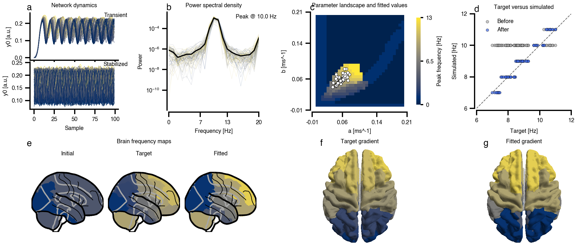
Jansen-Rit MEG frequency gradient optimization. Region-specific time constants fitted so the network reproduces a posterior-to-anterior peak-frequency gradient, with the target derived from the connectome’s own tract lengths. (a) Network dynamics. grid. The y0 trajectory of every region, shaded by node: the approach from the initial state, and the settled activity the spectra are computed from. (b) Power spectral density. line of integration__psd_frequencies (integration__simulated_psd), line of integration__psd_frequencies (integration__avg_spectrum) from experiment 1. Mean spectrum across regions; the alpha peak the fit moves region by region. (c) Parameter landscape and fitted values. JansenRit.b as a matrix (results), optimization__spectral_gradient_fit__fitted__dynamics__a as a matrix (optimization__spectral_gradient_fit__fitted__dynamics__b) from experiment 1. Peak frequency over the (a, b) plane, with each region’s fitted pair marked. (d) Target versus simulated. scatter of integration__target_peak_frequencies (integration__peak_frequencies), scatter of optimization__spectral_gradient_fit__observation__target_peak_frequencies (optimization__spectral_gradient_fit__observation__peak_frequencies) from experiment 1. Every region before and after the fit; the dashed line is agreement, and fitting collapses the cloud onto it. (e) Brain frequency maps. volume (integration__peak_frequencies), volume (integration__target_peak_frequencies), volume (optimization__spectral_gradient_fit__observation__peak_frequencies) from experiment 1. Initial, target and fitted peak frequency painted into the Desikan-Killiany volume. (f) Target gradient. surface (integration__target_peak_frequencies) from experiment 1. The target gradient on the fsaverage cortical surface. (g) Fitted gradient. surface (optimization__spectral_gradient_fit__observation__peak_frequencies) from experiment 1. The fitted gradient on the same surface and colour scale.
The fit descends the landscape in (c): only a narrow band of the \((a, b)\) plane oscillates at all, and the alpha band sits on its upper edge. (d) shows what the fit buys: the initial network rhythms almost uniformly, while the fitted map reproduces the posterior-to-anterior gradient of the target. (f) and (g) are that same comparison on the cortical surface.
Peak frequency here is read as the argmax of a Welch spectrum over a 1 s window, which quantises it to roughly 1 Hz. That resolution, not the optimiser, sets the floor on how closely the fitted points in (d) can sit on the target line.
See also
Model fitting: how losses and gradients work in TVBO.
K. Mahjoory, J.-M. Schoffelen, A. Keitel, and J. Gross, “The frequency gradient of human resting-state brain oscillations follows cortical hierarchies,”eLife, vol. 9, p. e53715, 2020, doi: 10.7554/eLife.53715.