import yamlfrom tvbo import Dynamics, SimulationExperimentfrom tvbo.datamodel.schema import Integrator# Pendulum Systempendulum_dynamics ="""name: PendulumSystemdescription: A simple damped pendulum system for demonstrating TVBO capabilities.parameters: c: description: Damping coefficient value: 0.001 unit: 1/ms omega0: description: Natural frequency value: 0.01 unit: rad/ms L: description: Length of the pendulum unit: m value: 1.0state_variables: theta: description: Angle of the pendulum unit: rad initial_value: 1.0 equation: rhs: omega omega: description: Angular velocity unit: rad/ms initial_value: 0.0 equation: rhs: -c*omega - omega0**2 * sin(theta)derived_variables: x: description: X coordinate of the pendulum bob unit: m equation: rhs: L * sin(theta) y: description: Y coordinate of the pendulum bob unit: m equation: rhs: -L * cos(theta)output: - x - y"""pendulum = SimulationExperiment( dynamics=Dynamics.from_string(pendulum_dynamics),# This pendulum swings with a period near 630 ms, so 0.1 ms resolves it finely. Left unset the step defaults to 0.0122 ms, which is sized for neural masses and puts fifty thousand steps in every swing. integration=Integrator(step_size=0.1),)results = pendulum.run('tvboptim', duration=5_000)
* Owlready2 * Warning: ignoring cyclic subclass of/subproperty of, involving:
  http://uri.interlex.org/tgbugs/uris/readable/atlas/Space

INFO [tvbo.run] [+0s] STEP 1: Running simulation...
INFO [tvbo.run] [+1s]   Simulation period: 5000.0 ms, dt: 0.1 ms
INFO [tvbo.run] [+1s]   Simulation complete.
INFO [tvbo.run] [+1s] Experiment complete.
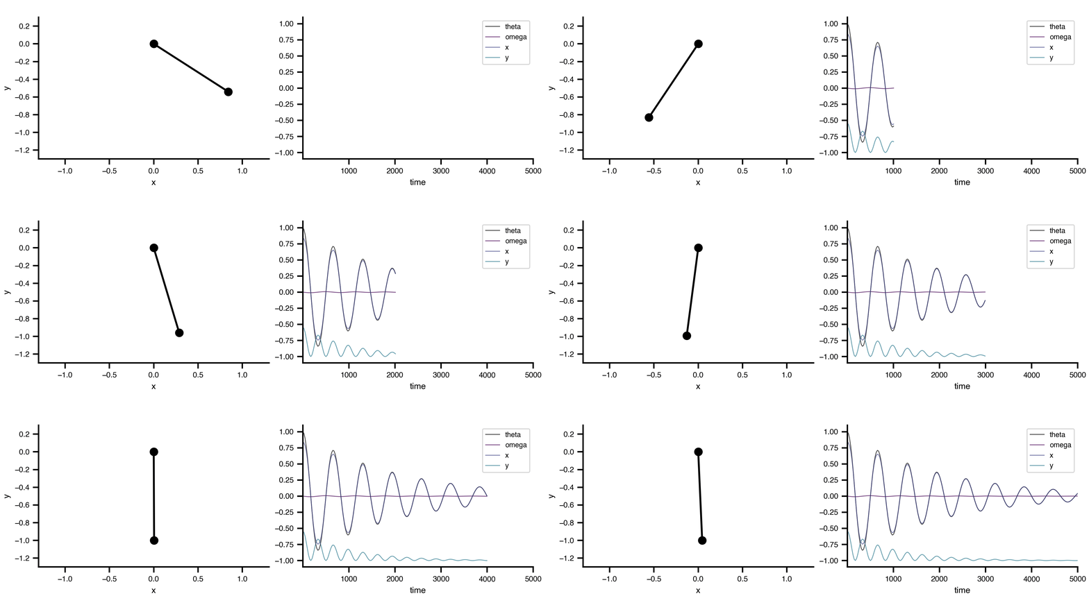
Real-time animation of the pendulum motion alongside the time series data:
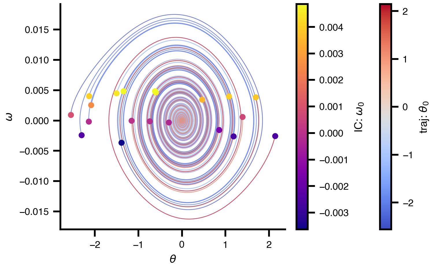
Phase Portrait
State variables accept a Distribution for initial conditions. The presence of a distribution declares that the variable should be sampled, with no runtime flags needed. The resolution order is:
Configuration
Behavior
initial_value: 1.0 (no distribution)
Deterministic; always starts at 1.0
distribution: present + n_trials > 1
Each trial samples a new IC from the distribution
distribution: present, single run
Uses initial_value as fallback
distribution.domain not set
Falls back to the state variable’s domain
# Case 1: Fixed IC (no distribution)theta:initial_value:1.0 # → Always starts at 1.0# Case 2: Sampled IC (distribution present)theta:initial_value:0.0 # fallback if sampling disableddistribution:name: Uniformdomain:{lo:-3.14,hi:3.14} # → Sampled when n_trials > 1, else uses 0.0# Case 3: Distribution without explicit domain → inherits SV domaintheta:initial_value:0.0domain:{lo:-3.14,hi:3.14}distribution:name: Uniform # domain falls back to SV domain # → Uniform(-3.14, 3.14)
An Exploration with n_trials runs them in parallel, and each trial samples a different starting point, revealing the full phase portrait without any Python loop:
from tvbo.datamodel.schema import Distribution, Range, Explorationimport numpy as np# Attach sampling distributions to the state variablespendulum.dynamics.state_variables["theta"].distribution = Distribution( name="Uniform", domain=Range(lo=-np.pi, hi=np.pi))pendulum.dynamics.state_variables["omega"].distribution = Distribution( name="Uniform", domain=Range(lo=-0.005,hi=0.005))# 20 parallel trials from different initial conditionspendulum.explorations["ICs"] = Exploration(name="ICs", n_trials=20)result = pendulum.run(duration=10_000)
INFO [tvbo.run] [+0s] STEP 1: Running simulation...
INFO [tvbo.run] [+1s]   Simulation period: 10000.0 ms, dt: 0.1 ms
INFO [tvbo.run] [+1s]   Simulation complete.
INFO [tvbo.run] [+1s] STEP 2: Running explorations...
INFO [tvbo.run] [+1s]   > ICs
INFO [tvbo.run] [+1s]   Explorations complete.
INFO [tvbo.run] [+1s] Experiment complete.
import numpy as npimport matplotlib.pyplot as pltdef plot_phase_portrait(trials, color_trajectory_by="theta", color_ic_by=None, cmap="coolwarm", ic_cmap=None, ax=None):"""Plot phase portrait with independent coloring for trajectories and ICs. color_trajectory_by: "theta" or "omega" — colors lines by that IC value color_ic_by: "theta" or "omega" — colors IC dots (None = black) """ label_map = {"theta": r"$\theta_0$", "omega": r"$\omega_0$"}if ax isNone: fig, ax = plt.subplots(figsize=(5, 4), layout="compressed")else: fig = ax.figure ax.set_box_aspect(1)# `trials` is a labelled DataArray with dims (trial, time, variable, node),# so every axis is selected by name — no positional indices to drift out of# sync if the intrinsic rank changes.## The exploration records the declared outputs (x, y). The pendulum geometry# is x = L sin(theta), y = -L cos(theta), so the phase-plane coordinates come# back exactly: theta = atan2(x, -y), and omega = d(theta)/dt. dt =float(trials.coords["time"].values[1] - trials.coords["time"].values[0])def state_of(tid): run = trials.sel(trial=tid) x = run.sel(variable="x").squeeze(drop=True).values y = run.sel(variable="y").squeeze(drop=True).values theta = np.unwrap(np.arctan2(x, -y)) omega = np.gradient(theta, dt)return theta, omega trial_ids = trials.coords["trial"].values states = {int(t): state_of(t) for t in trial_ids} var_pos = {"theta": 0, "omega": 1}def ic_of(var):"""Initial value of `var` for each trial.""" k = var_pos[var]return np.array([states[int(t)][k][0] for t in trial_ids])# Trajectory colors traj_ics = ic_of(color_trajectory_by) traj_norm = plt.Normalize(float(traj_ics.min()), float(traj_ics.max())) traj_cm = plt.colormaps[cmap]# IC dot colorsif color_ic_by isnotNone: ic_vals = ic_of(color_ic_by) ic_norm = plt.Normalize(float(ic_vals.min()), float(ic_vals.max())) ic_cm = plt.colormaps[ic_cmap or cmap]for i, tid inenumerate(trial_ids): theta, omega = states[int(tid)] ax.plot(theta, omega, lw=0.6, alpha=0.7, color=traj_cm(traj_norm(traj_ics[i]))) dot_color = ic_cm(ic_norm(ic_vals[i])) if color_ic_by else"black" ax.plot(theta[0], omega[0], "o", ms=4, color=dot_color, zorder=5)# Colorbars sm = plt.cm.ScalarMappable(cmap=traj_cm, norm=traj_norm) fig.colorbar(sm, ax=ax, label=f"traj: {label_map[color_trajectory_by]}")if color_ic_by isnotNone: sm2 = plt.cm.ScalarMappable(cmap=ic_cm, norm=ic_norm) fig.colorbar(sm2, ax=ax, label=f"IC: {label_map[color_ic_by]}") ax.set_xlabel(r"$\theta$") ax.set_ylabel(r"$\omega$") plt.close()return figtrials = result.exploration.ICs.as_grid() # labelled: (trial, time, variable, node)plot_phase_portrait(trials, color_trajectory_by="theta", color_ic_by="omega", cmap="coolwarm", ic_cmap="plasma")