PyRates Parameter Analysis

This guide demonstrates how to use TVBO models with PyRates for parameter sweeps and sensitivity analysis.

Overview

PyRates provides powerful tools for parameter analysis:

• Grid Search: Simulate multiple parameter combinations in parallel
• Parameter Sweeps: 1D/2D exploration of parameter space
• Sensitivity Analysis: Identify critical parameters

The workflow:

1. Define model in TVBO
2. Export to PyRates format
3. Run parameter sweeps using PyRates grid_search()
4. Analyze and visualize results

Setup

import os
import shutil
import numpy as np
import matplotlib.pyplot as plt
from matplotlib import cm
from pyrates import grid_search, CircuitTemplate, clear

Example 1: Van der Pol Parameter Sweep

Explore how the damping parameter μ affects oscillation behavior.

Define Model in TVBO

from tvbo import Dynamics
from IPython.display import Markdown, display

# Create Van der Pol oscillator
vdp = Dynamics("Dynamics")
vdp.name = "VdP"
vdp.add_parameter("mu", value=1.0, description="Damping parameter")
vdp.add_state_variable("x", equation="z", initial_value=0.1)
vdp.add_state_variable("z", equation="mu*(1 - x**2)*z - x", initial_value=0.0)

# Display model summary using generate_report
display(Markdown(vdp.generate_report(format="markdown")))

VdP

State Equations

\[ \frac{d}{d t} x = z \] \[ \frac{d}{d t} z = - x + \mu*z*\left(1 - x^{2}\right) \]

Parameters

Parameter	Value	Unit	Description
\(\mu\)	1.0	N/A	Damping parameter

Export to PyRates

# Create module directory
os.makedirs('_sweep_vdp', exist_ok=True)
with open('_sweep_vdp/__init__.py', 'w') as f:
    f.write('')

# Export
vdp.to_yaml(format="pyrates", filepath='_sweep_vdp/model.yaml')

print("Model exported to _sweep_vdp/model.yaml")

Model exported to _sweep_vdp/model.yaml

Run Parameter Sweep

# Define parameter grid
mu_values = [0.1, 0.5, 1.0, 2.0, 5.0, 10.0]
param_grid = {'mu': mu_values}

# Map parameters to model variables
param_map = {
    'mu': {'vars': ['VdP_op/mu'], 'nodes': ['p']}
}

# Simulation settings
T = 100.0
dt = 1e-3
dts = 1e-2

# Run grid search
print("Running parameter sweep...")
results, results_map = grid_search(
    circuit_template='_sweep_vdp.model.VdP_circuit',
    param_grid=param_grid,
    param_map=param_map,
    simulation_time=T,
    step_size=dt,
    sampling_step_size=dts,
    outputs={'x': 'p/VdP_op/x', 'z': 'p/VdP_op/z'},
    solver='scipy',
    backend='default',
    clear=True
)

print(f"Sweep complete! Results shape: {results.shape}")
print(f"Results map: {results_map}")

Running parameter sweep...
Compilation Progress
--------------------
    (1) Translating the circuit template into a networkx graph representation...
        ...finished.
    (2) Preprocessing edge transmission operations...
        ...finished.
    (3) Parsing the model equations into a compute graph...
        ...finished.
    Model compilation was finished.
Simulation Progress
-------------------
     (1) Generating the network run function...
     (2) Processing output variables...
        ...finished.
     (3) Running the simulation...
        ...finished after 0.04460929200286046s.
Sweep complete! Results shape: (10000, 12)
Results map:                  mu
VdP_circuit_0   0.1
VdP_circuit_1   0.5
VdP_circuit_2   1.0
VdP_circuit_3   2.0
VdP_circuit_4   5.0
VdP_circuit_5  10.0

Visualize Results

# Time series for different μ values
fig, axes = plt.subplots(2, 3, figsize=(14, 8))
axes = axes.flatten()

time = results.index

# Get x and z columns - they are ordered by parameter index
x_cols = [c for c in results.columns if c[0] == 'x']
z_cols = [c for c in results.columns if c[0] == 'z']

for i, mu in enumerate(mu_values):
    ax = axes[i]

    # Columns are indexed by circuit instance number
    x_col = x_cols[i]
    z_col = z_cols[i]

    ax.plot(time, results[x_col], label='x')
    ax.plot(time, results[z_col], alpha=0.7, label='z')
    ax.set_title(f'μ = {mu}')
    ax.set_xlabel('Time (ms)')
    ax.set_ylabel('State')
    ax.legend(loc='upper right')
    ax.set_xlim([0, T])

plt.tight_layout()
plt.suptitle('Van der Pol Oscillator: Effect of Damping (μ)', y=1.02)
plt.show()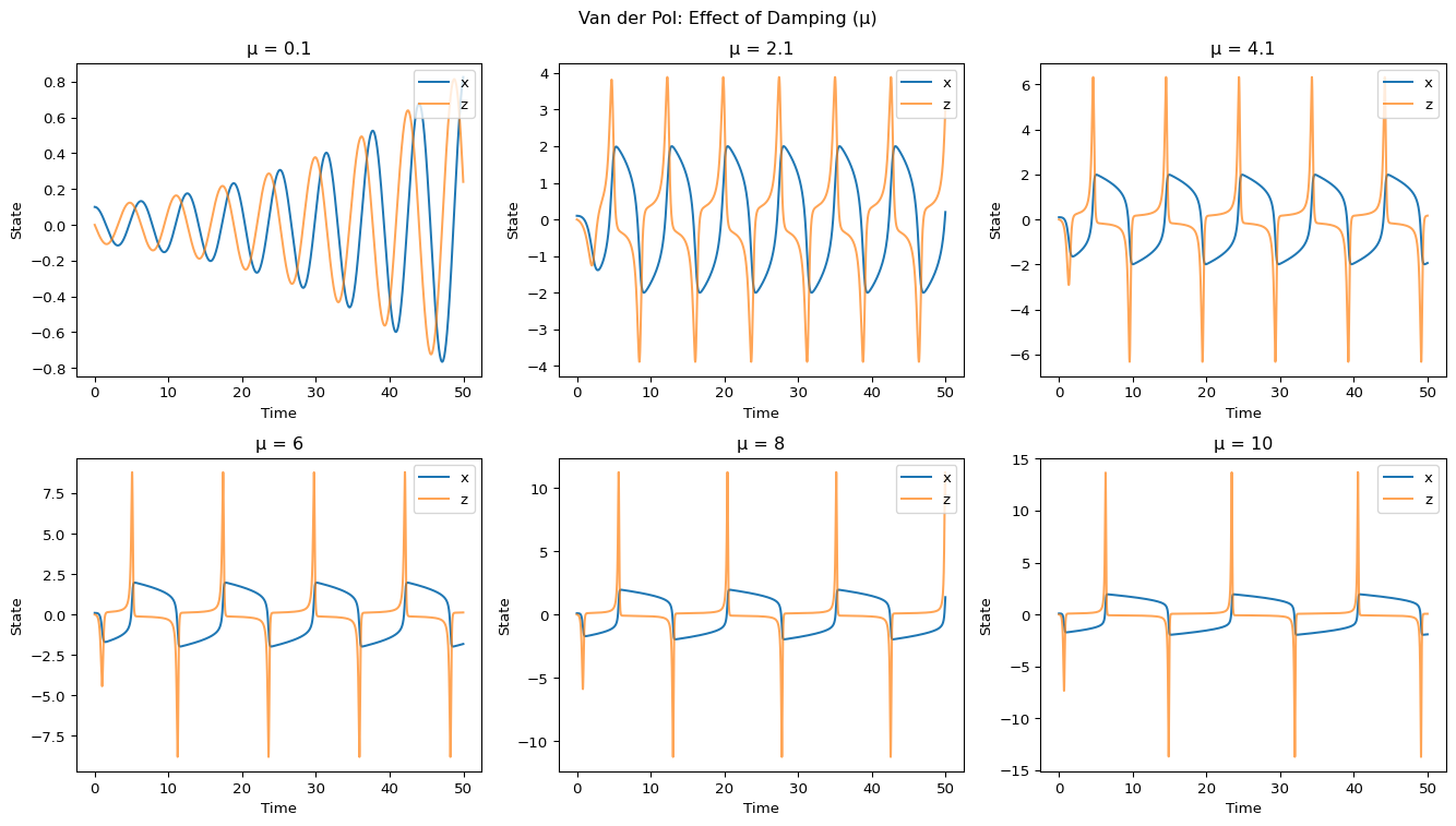

Phase Space Analysis

# Phase portraits for different μ values
fig, axes = plt.subplots(2, 3, figsize=(14, 8))
axes = axes.flatten()

colors = cm.viridis(np.linspace(0, 1, len(mu_values)))

for i, mu in enumerate(mu_values):
    ax = axes[i]
    x_col = x_cols[i]
    z_col = z_cols[i]

    x = results[x_col].values
    z = results[z_col].values

    ax.plot(x, z, color=colors[i], linewidth=0.5)
    ax.scatter(x[0], z[0], color='green', s=50, zorder=5, label='Start')
    ax.scatter(x[-1], z[-1], color='red', s=50, zorder=5, label='End')
    ax.set_title(f'μ = {mu}')
    ax.set_xlabel('x')
    ax.set_ylabel('z')
    ax.set_box_aspect(1)

plt.tight_layout()
plt.suptitle('Van der Pol Phase Portraits', y=1.02)
plt.show()

# Cleanup
shutil.rmtree('_sweep_vdp')

Example 2: 2D Parameter Sweep

Explore two parameters simultaneously.

Define FitzHugh-Nagumo Model

from tvbo import Dynamics
from IPython.display import Markdown, display

# FitzHugh-Nagumo model
fhn = Dynamics("Dynamics")
fhn.name = "FHN"
fhn.add_parameter("a", value=0.7)
fhn.add_parameter("b", value=0.8)
fhn.add_parameter("tau", value=12.5)
fhn.add_parameter("I_ext", value=0.5)

fhn.add_state_variable("v", equation="v - v**3/3 - w + I_ext", initial_value=0.0)
fhn.add_state_variable("w", equation="(v + a - b*w)/tau", initial_value=0.0)

# Display model summary using generate_report
display(Markdown(fhn.generate_report(format="markdown")))

# Also show the generated Python code
print("=== Generated Python Code ===")
print(fhn.render_code(format="python"))

FHN

State Equations

\[ \frac{d}{d t} v = I_{ext} + v - w - \frac{v^{3}}{3} \] \[ \frac{d}{d t} w = \frac{a + v - b*w}{\tau} \]

Parameters

Parameter	Value	Unit	Description
\(a\)	0.7	N/A	None
\(b\)	0.8	N/A	None
\(\tau\)	12.5	N/A	None
\(I_{ext}\)	0.5	N/A	None

=== Generated Python Code ===
import numpy as np
import scipy


def FHN(
    current_state,
    t,
    a=0.7,
    b=0.8,
    tau=12.5,
    I_ext=0.5,
    local_coupling=0.0,
    stimulus=None,
    stimulus_scaling=1.0,
):
    e = np.e
    stim_t = stimulus_scaling * stimulus(t) if stimulus is not None else 0.0

    v = current_state[0]
    w = current_state[1]

    # Derived Variables

    # Time Derivatives
    next_state = np.array(
        [
            # v
            I_ext + v - w - 1 / 3 * v**3,
            # w
            (a + v - b * w) / tau,
        ]
    )

    return next_state

2D Grid Search via Sequential Sweeps

PyRates grid_search performs 1D sweeps efficiently. For 2D parameter exploration, we run sequential sweeps, varying one parameter while fixing the other.

# Export model
os.makedirs('_sweep_fhn', exist_ok=True)
with open('_sweep_fhn/__init__.py', 'w') as f:
    f.write('')
fhn.to_yaml(format="pyrates", filepath='_sweep_fhn/model.yaml')

# Parameter values
a_values = np.linspace(0.5, 1.0, 5)
I_values = np.linspace(0.0, 1.0, 5)

# Simulation settings
T = 200.0
dt = 1e-3
dts = 1e-1

# Store amplitudes for 2D heatmap
amplitudes = np.zeros((len(a_values), len(I_values)))

print("Running 2D parameter sweep via sequential 1D sweeps...")

# For each value of 'a', sweep over I_ext
for i, a_val in enumerate(a_values):
    # Update model with fixed 'a' value
    fhn_temp = Dynamics("Dynamics")
    fhn_temp.name = "FHN"
    fhn_temp.add_parameter("a", value=a_val)
    fhn_temp.add_parameter("b", value=0.8)
    fhn_temp.add_parameter("tau", value=12.5)
    fhn_temp.add_parameter("I_ext", value=0.5)
    fhn_temp.add_state_variable("v", equation="v - v**3/3 - w + I_ext", initial_value=0.0)
    fhn_temp.add_state_variable("w", equation="(v + a - b*w)/tau", initial_value=0.0)
    fhn_temp.to_yaml(format="pyrates", filepath='_sweep_fhn/model.yaml')

    # 1D sweep over I_ext
    param_grid = {'I': I_values.tolist()}
    param_map = {'I': {'vars': ['FHN_op/I_ext'], 'nodes': ['p']}}

    results, _ = grid_search(
        circuit_template='_sweep_fhn.model.FHN_circuit',
        param_grid=param_grid,
        param_map=param_map,
        simulation_time=T,
        step_size=dt,
        sampling_step_size=dts,
        outputs={'v': 'p/FHN_op/v'},
        solver='scipy',
        backend='default',
        clear=True
    )

    # Extract amplitudes for each I value
    v_cols = list(results.columns)
    for j in range(len(I_values)):
        v = results[v_cols[j]].values
        v_steady = v[len(v)//2:]  # Use second half
        amplitudes[i, j] = np.max(v_steady) - np.min(v_steady)

    print(f"  a = {a_val:.2f} complete")

print("2D sweep complete!")

Running 2D parameter sweep via sequential 1D sweeps...
Compilation Progress
--------------------
    (1) Translating the circuit template into a networkx graph representation...
        ...finished.
    (2) Preprocessing edge transmission operations...
        ...finished.
    (3) Parsing the model equations into a compute graph...
        ...finished.
    Model compilation was finished.
Simulation Progress
-------------------
     (1) Generating the network run function...
     (2) Processing output variables...
        ...finished.
     (3) Running the simulation...
        ...finished after 0.02142716700109304s.
  a = 0.50 complete
Compilation Progress
--------------------
    (1) Translating the circuit template into a networkx graph representation...
        ...finished.
    (2) Preprocessing edge transmission operations...
        ...finished.
    (3) Parsing the model equations into a compute graph...
        ...finished.
    Model compilation was finished.
Simulation Progress
-------------------
     (1) Generating the network run function...
     (2) Processing output variables...
        ...finished.
     (3) Running the simulation...
        ...finished after 0.02562937499897089s.
  a = 0.62 complete
Compilation Progress
--------------------
    (1) Translating the circuit template into a networkx graph representation...
        ...finished.
    (2) Preprocessing edge transmission operations...
        ...finished.
    (3) Parsing the model equations into a compute graph...
        ...finished.
    Model compilation was finished.
Simulation Progress
-------------------
     (1) Generating the network run function...
     (2) Processing output variables...
        ...finished.
     (3) Running the simulation...
        ...finished after 0.02302974999838625s.
  a = 0.75 complete
Compilation Progress
--------------------
    (1) Translating the circuit template into a networkx graph representation...
        ...finished.
    (2) Preprocessing edge transmission operations...
        ...finished.
    (3) Parsing the model equations into a compute graph...
        ...finished.
    Model compilation was finished.
Simulation Progress
-------------------
     (1) Generating the network run function...
     (2) Processing output variables...
        ...finished.
     (3) Running the simulation...
        ...finished after 0.021144875001482433s.
  a = 0.88 complete
Compilation Progress
--------------------
    (1) Translating the circuit template into a networkx graph representation...
        ...finished.
    (2) Preprocessing edge transmission operations...
        ...finished.
    (3) Parsing the model equations into a compute graph...
        ...finished.
    Model compilation was finished.
Simulation Progress
-------------------
     (1) Generating the network run function...
     (2) Processing output variables...
        ...finished.
     (3) Running the simulation...
        ...finished after 0.025597792002372444s.
  a = 1.00 complete
2D sweep complete!

Amplitude Analysis

# Plot heatmap
fig, ax = plt.subplots(figsize=(8, 6))
im = ax.imshow(amplitudes, origin='lower', aspect='auto',
               extent=[I_values[0], I_values[-1], a_values[0], a_values[-1]],
               cmap='viridis')
ax.set_xlabel('External Current (I_ext)')
ax.set_ylabel('Parameter a')
ax.set_title('FitzHugh-Nagumo: Oscillation Amplitude')
plt.colorbar(im, ax=ax, label='Amplitude')
plt.tight_layout()
plt.show()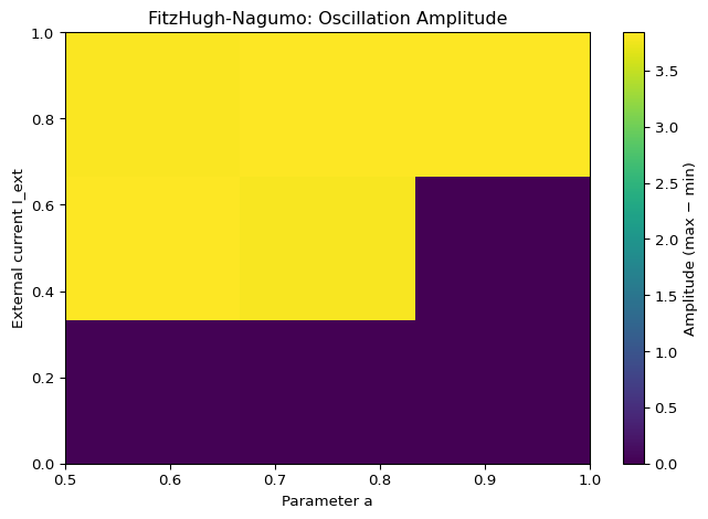

# Cleanup
shutil.rmtree('_sweep_fhn')

Example 3: Bifurcation-like Analysis

Detect qualitative changes in dynamics across parameter range.

QIF Neural Mass Model

from tvbo import Dynamics
from IPython.display import Markdown, display

# Quadratic Integrate-and-Fire mean-field model
qif = Dynamics("Dynamics")
qif.name = "QIF"

# Parameters
qif.add_parameter("tau", value=1.0)
qif.add_parameter("eta", value=-5.0)  # Background drive
qif.add_parameter("J", value=15.0)    # Coupling strength
qif.add_parameter("Delta", value=1.0)  # Heterogeneity

# State variables
qif.add_state_variable("r", equation="Delta/(tau*pi) + 2*r*v", initial_value=0.1)
qif.add_state_variable("v", equation="v**2 + eta + J*r*tau - (pi*r*tau)**2", initial_value=-2.0)

# Display model summary using generate_report
display(Markdown(qif.generate_report(format="markdown")))

QIF

State Equations

\[ \frac{d}{d t} r = 2*r*v + \frac{\Delta}{\pi*\tau} \] \[ \frac{d}{d t} v = \eta + v^{2} + J*r*\tau - \pi^{2}*r^{2}*\tau^{2} \]

Parameters

Parameter	Value	Unit	Description
\(\tau\)	1.0	N/A	None
\(\eta\)	-5.0	N/A	None
\(J\)	15.0	N/A	None
\(\Delta\)	1.0	N/A	None

Sweep Over η (Background Drive)

# Export
os.makedirs('_sweep_qif', exist_ok=True)
with open('_sweep_qif/__init__.py', 'w') as f:
    f.write('')
qif.to_yaml(format="pyrates", filepath='_sweep_qif/model.yaml')

# Parameter grid
eta_values = np.linspace(-10, 5, 30)

param_grid = {'eta': eta_values.tolist()}
param_map = {'eta': {'vars': ['QIF_op/eta'], 'nodes': ['p']}}

# Long simulation to find steady states
T = 500.0
dt = 1e-3
dts = 1e-1

print("Running bifurcation-like sweep...")
results_qif, results_map_qif = grid_search(
    circuit_template='_sweep_qif.model.QIF_circuit',
    param_grid=param_grid,
    param_map=param_map,
    simulation_time=T,
    step_size=dt,
    sampling_step_size=dts,
    outputs={'r': 'p/QIF_op/r'},
    solver='scipy',
    backend='default',
    clear=True
)

print(f"Sweep complete! Results shape: {results_qif.shape}")

Running bifurcation-like sweep...
Compilation Progress
--------------------
    (1) Translating the circuit template into a networkx graph representation...
        ...finished.
    (2) Preprocessing edge transmission operations...
        ...finished.
    (3) Parsing the model equations into a compute graph...
        ...finished.
    Model compilation was finished.
Simulation Progress
-------------------
     (1) Generating the network run function...
     (2) Processing output variables...
        ...finished.
     (3) Running the simulation...
        ...finished after 0.27347316599843907s.
Sweep complete! Results shape: (5000, 30)

Bifurcation-like Diagram

fig, axes = plt.subplots(1, 2, figsize=(14, 5))

# Get all r columns
r_cols = list(results_qif.columns)

# Extract steady-state firing rates
r_min = []
r_max = []
r_mean = []

for i, eta in enumerate(eta_values):
    r = results_qif[r_cols[i]].values

    # Use last 20% for steady state
    r_steady = r[int(0.8*len(r)):]
    r_min.append(np.min(r_steady))
    r_max.append(np.max(r_steady))
    r_mean.append(np.mean(r_steady))

# Bifurcation-like diagram
ax = axes[0]
ax.fill_between(eta_values, r_min, r_max, alpha=0.3, label='Oscillation range')
ax.plot(eta_values, r_mean, 'k-', linewidth=2, label='Mean firing rate')
ax.set_xlabel('η (Background drive)')
ax.set_ylabel('Firing rate r')
ax.set_title('QIF Model: Bifurcation-like Diagram')
ax.legend()
ax.grid(True, alpha=0.3)

# Select sample traces
ax = axes[1]
sample_indices = [0, 10, 15, 25]  # Indices into eta_values
colors = plt.cm.viridis(np.linspace(0, 1, len(sample_indices)))

for idx, color in zip(sample_indices, colors):
    eta = eta_values[idx]
    r = results_qif[r_cols[idx]].values
    t = results_qif.index.values
    start_idx = int(0.6 * len(r))

    ax.plot(t[start_idx:] - t[start_idx], r[start_idx:],
            color=color, label=f'η = {eta:.1f}')

ax.set_xlabel('Time (ms)')
ax.set_ylabel('Firing rate r')
ax.set_title('Sample Time Series')
ax.legend()

plt.tight_layout()
plt.show()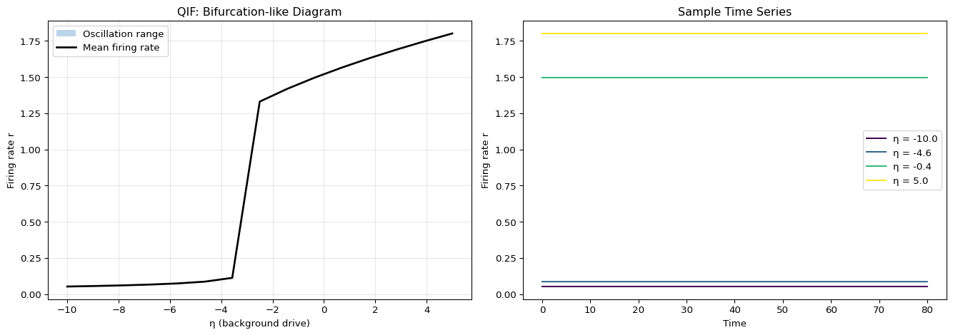

# Cleanup
shutil.rmtree('_sweep_qif')

Summary

TVBO enables seamless integration with PyRates parameter analysis:

1. Define models in TVBO’s structured format
2. Export to PyRates with model.to_yaml(format="pyrates")
3. Analyze using PyRates grid_search() for parallel parameter sweeps
4. Visualize results to understand parameter effects

Key Functions

from pyrates import grid_search

results, results_map = grid_search(
    circuit_template='module.file.circuit_name',
    param_grid={'param': [values]},          # Parameter combinations
    param_map={'param': {'vars': ['op/var'], 'nodes': ['node']}},
    simulation_time=T,
    step_size=dt,
    sampling_step_size=dts,
    outputs={'name': 'node/op/var'},
    solver='scipy',
    backend='default'
)

Next Steps

• PyRates Bifurcation: Numerical continuation and bifurcation detection
• PyRates Interoperability: Basic round-trip examples