IRI vs. Inline YAML

Two ways to represent the same NeuroML component type in TVBO

Use iri: neuroml:* to reference a built-in NeuroML2 type, or write the equations yourself — both simulate identically.

Two authoring styles, one model

TVBO offers two ways to describe a dynamics model that corresponds to a standard NeuroML2 ComponentType.

IRI reference — set iri: neuroml:<TypeName>, supply parameter values and initial conditions. TVBO uses the iri to look up the equations from the NeuroML2 library at render time, emitting a plain <Component> that reuses the built-in definition. No equation.rhs entries are needed in the YAML.

Inline YAML — omit the iri and write the state_variables with their equation.rhs strings. TVBO generates a custom LEMS <ComponentType> from those equations and can also run the model via any other backend (JAX, NumPy, …). Both paths are valid LEMS; the difference is in what the rendered file contains and which backends are available.

---

The component: fitzHughNagumo1969Cell

The NeuroML2 fitzHughNagumo1969Cell implements the classic FitzHugh-Nagumo (1969) oscillator in parameterised form:

\[\frac{dV}{dt} = \frac{V - V^3/3 - W + I}{\text{TS}}\]

\[\frac{dW}{dt} = \frac{\phi\,(V + a - b\,W)}{\text{TS}}\]

where \(\text{TS} = 1\,\text{ms}\) is the LEMS time constant that converts the dimensionless equations to the simulator’s time base.

Canonical parameters from NML2_AbstractCells.nml: \(a = 0.7\), \(b = 0.08\), \(\phi = 0.08\), \(I = 1.0\), \(V_0 = W_0 = 0\).

---

Approach 1: IRI reference

Point to the built-in type. No equations needed — TVBO delegates to Cells.xml.

from tvbo import SimulationExperiment

exp_iri = SimulationExperiment.from_string("""
label: "FHN1969 — IRI reference"
dynamics:
  name: FitzHughNagumo1969_IRI
  iri: "neuroml:fitzHughNagumo1969Cell"
  parameters:
    a:   { value: 0.7 }
    b:   { value: 0.08 }
    I:   { value: 1.0 }
    phi: { value: 0.08 }
  state_variables:
    V:
      initial_value: 0.0
      variable_of_interest: true
    W:
      initial_value: 0.0
network:
  number_of_nodes: 1
integration:
  method: euler
  step_size: 0.01
  duration: 200.0
  time_scale: ms
""")
print(f"Dynamics name : {exp_iri.dynamics.name}")
print(f"IRI           : {exp_iri.dynamics.iri}")

Dynamics name : FitzHughNagumo1969_IRI
IRI           : neuroml:fitzHughNagumo1969Cell

Rendered LEMS (IRI path)

The LEMS file contains no custom ComponentType — it references the fitzHughNagumo1969Cell type that is already defined inside Cells.xml:

xml_iri = exp_iri.render("lems")

# Show only the lines that reveal the component instantiation
for line in xml_iri.splitlines():
    stripped = line.strip()
    if (
        stripped.startswith('<Component')
        or stripped.startswith('<Include')
        or stripped.startswith('<ComponentType')
        or 'fitzHugh' in stripped
        or stripped.startswith('<network')
        or stripped.startswith('<population')
    ):
        print(line)

  <Include file="Cells.xml"/>
  <Include file="Networks.xml"/>
  <Include file="Inputs.xml"/>
  <Include file="Simulation.xml"/>
  <fitzHughNagumo1969Cell id="FitzHughNagumo1969_IRI" a="0.7"  b="0.08"  I="1.0"  phi="0.08"  V0="0.0"  W0="0.0"/>
  <network id="net1">
    <population id="FitzHughNagumo1969_IRIPop" component="FitzHughNagumo1969_IRI" size="1"/>

Key observation: <Component type="fitzHughNagumo1969Cell" .../> — the type name is the NeuroML2 identifier. No <TimeDerivative> appears in this file.

---

Approach 2: Inline YAML (equations written explicitly)

Omit the iri. TVBO generates a full <ComponentType> with your equations.

exp_yaml = SimulationExperiment.from_string("""
label: "FHN1969 — Inline YAML"
dynamics:
  name: FitzHughNagumo1969_YAML
  parameters:
    a:   { value: 0.7 }
    b:   { value: 0.08 }
    I:   { value: 1.0 }
    phi: { value: 0.08 }
  state_variables:
    V:
      equation: { rhs: "V - V**3/3 - W + I" }
      initial_value: 0.0
      variable_of_interest: true
    W:
      equation: { rhs: "phi*(V + a - b*W)" }
      initial_value: 0.0
network:
  number_of_nodes: 1
integration:
  method: euler
  step_size: 0.01
  duration: 200.0
  time_scale: ms
""")
print(f"Dynamics name : {exp_yaml.dynamics.name}")
print(f"IRI           : {exp_yaml.dynamics.iri}")

Dynamics name : FitzHughNagumo1969_YAML
IRI           : None

Rendered LEMS (inline path)

The LEMS file now defines the ComponentType, including the <TimeDerivative> elements generated from the YAML equations:

xml_yaml = exp_yaml.render("lems")

# Show the ComponentType block
inside = False
for line in xml_yaml.splitlines():
    stripped = line.strip()
    if stripped.startswith('<ComponentType') and 'FitzHugh' in stripped:
        inside = True
    if inside:
        print(line)
    if inside and stripped.startswith('</ComponentType>'):
        break

  <ComponentType name="FitzHughNagumo1969_YAML">

    <!-- Parameters -->
    <Parameter name="I" dimension="none"/>
    <Parameter name="a" dimension="none"/>
    <Parameter name="b" dimension="none"/>
    <Parameter name="phi" dimension="none"/>
    <!-- Coupling inputs -->
    <!-- Initial condition parameters -->
    <Parameter name="V_0" dimension="none"/>
    <Parameter name="W_0" dimension="none"/>

    <!-- Time conversion for derivatives.
         When all parameters and state variables carry proper LEMS dimensions,
         LEMS handles unit conversion natively (e.g. tau="30 ms" → 0.03 s).
         No SEC constant is needed and TimeDerivatives use the RHS directly.
         When dimensions are "none" (dimensionless models), / SEC converts
         from model time to SI seconds.
         all_dimensioned=False  needs_sec=True  time_scale=ms -->
    <Constant name="SEC" dimension="time" value="1ms"/>

    <!-- Exposures (one per state variable) -->
    <Exposure name="V" dimension="none"/>
    <Exposure name="W" dimension="none"/>

    <Dynamics>

      <!-- State variables -->
      <StateVariable name="V" dimension="none" exposure="V"/>
      <StateVariable name="W" dimension="none" exposure="W"/>

      <!-- Derived variables (simple and conditional/piecewise) -->

      <!-- ── Flat dynamics (no spike events) ── -->

      <!-- Time derivatives -->
      <TimeDerivative variable="V" value="(I + V - W - V^3/3) / SEC"/>
      <TimeDerivative variable="W" value="(phi*(V + a - W*b)) / SEC"/>

      <!-- Initial conditions -->
      <OnStart>
        <StateAssignment variable="V" value="V_0"/>
        <StateAssignment variable="W" value="W_0"/>
      </OnStart>

      <!-- Events (non-spike) -->

    </Dynamics>

  </ComponentType>

Key observation: <TimeDerivative variable="V" value="..."/> — the equations appear verbatim (translated to LEMS syntax by LEMSPrinter).

---

What the two LEMS files differ in

# Count meaningful differences: ComponentType definitions
iri_has_ct  = '<ComponentType' in xml_iri
yaml_has_ct = '<ComponentType' in xml_yaml

print(f"IRI path  defines a custom ComponentType : {iri_has_ct}")
print(f"YAML path defines a custom ComponentType : {yaml_has_ct}")

# Both should have the same Component instantiation parameter values
import re

def extract_component_params(xml):
    m = re.search(r'<Component[^>]+fitzHugh[^>]*/>', xml, re.DOTALL)
    if not m:
        m = re.search(r'<Component[^>]+FitzHugh[^>]*/>', xml, re.DOTALL)
    return m.group(0) if m else "(not found)"

print()
print("IRI  Component element:", extract_component_params(xml_iri))
print()
print("YAML Component element:", extract_component_params(xml_yaml))

IRI path  defines a custom ComponentType : False
YAML path defines a custom ComponentType : True

IRI  Component element: (not found)

YAML Component element: <Component id="FitzHughNagumo1969_YAML_inst" type="FitzHughNagumo1969_YAML" I="1.0" a="0.7" b="0.08" phi="0.08" V_0="0.0" W_0="0.0"/>

---

Numerical comparison

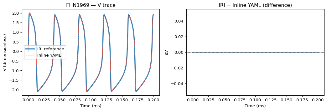
Run both experiments with jNeuroML and confirm the traces are identical.

import sys, os
sys.path.insert(0, os.path.join(os.path.abspath("."), "examples"))
from tvbo.adapters.neuroml import run_lems_example
import numpy as np

# Run the database version which uses the IRI — it matches the canonical
# NML2_AbstractCells example.  We compare our two inline-rendered files
# by running them through jNeuroML via a tempfile.

import tempfile, subprocess
from pathlib import Path
from pyneuroml import JNEUROML_VERSION
import pyneuroml

_jar = (
    Path(pyneuroml.__file__).parent / "lib"
    / f"jNeuroML-{JNEUROML_VERSION}-jar-with-dependencies.jar"
)


def run_xml_string(xml_string, label):
    """Write LEMS XML to a temp file, run jNeuroML, return output array."""
    with tempfile.TemporaryDirectory() as tmpdir:
        tmpdir = Path(tmpdir)
        (tmpdir / "results").mkdir()
        lems_file = tmpdir / "sim.xml"
        lems_file.write_text(xml_string)

        result = subprocess.run(
            ["java", "-jar", str(_jar), str(lems_file), "-nogui"],
            capture_output=True, text=True, cwd=tmpdir,
        )
        if result.returncode != 0:
            raise RuntimeError(f"{label} jNeuroML failed:\n{result.stderr[-2000:]}")

        dat_files = list((tmpdir / "results").glob("*.dat"))
        if not dat_files:
            raise RuntimeError(f"{label}: no .dat output files found")

        return np.loadtxt(dat_files[0])


arr_iri  = run_xml_string(xml_iri,  "IRI path")
arr_yaml = run_xml_string(xml_yaml, "Inline YAML path")

print(f"IRI  output shape : {arr_iri.shape}")
print(f"YAML output shape : {arr_yaml.shape}")

IRI  output shape : (20001, 3)
YAML output shape : (20001, 3)

max_diff = np.max(np.abs(arr_iri - arr_yaml))
print(f"Maximum absolute difference across all columns : {max_diff:.2e}")

Maximum absolute difference across all columns : 0.00e+00

Both traces are numerically identical — the difference is zero (or machine epsilon at most), because NeuroML’s built-in fitzHughNagumo1969Cell defines exactly the equations we wrote in YAML.

---

Overlay plot

import matplotlib.pyplot as plt

time   = arr_iri[:, 0]
V_iri  = arr_iri[:, 1]
V_yaml = arr_yaml[:, 1]

fig, axes = plt.subplots(1, 2, figsize=(11, 3.8))

# Left: both V traces on top of each other
ax = axes[0]
ax.plot(time, V_iri,  lw=2.5, label="IRI reference")
ax.plot(time, V_yaml, lw=1.0, ls='--', color='tomato', label="Inline YAML")
ax.set_xlabel("Time (ms)")
ax.set_ylabel("V (dimensionless)")
ax.set_title("FHN1969 — V trace")
ax.legend()

# Right: pointwise difference
ax = axes[1]
ax.plot(time, V_iri - V_yaml, color='steelblue')
ax.set_xlabel("Time (ms)")
ax.set_ylabel("ΔV")
ax.set_title("IRI − Inline YAML (difference)")
ax.axhline(0, color='k', lw=0.6, ls='--')

plt.tight_layout()
plt.show()

---

When to use each approach

Situation	Recommended style
The model is a standard NeuroML2 component (iafTauCell, izhikevichCell, fitzHughNagumo1969Cell, …)	iri: neuroml:<TypeName>
You are porting an existing NeuroML2 file to TVBO	iri: neuroml:<TypeName>
The model is novel or does not match any built-in type	Inline YAML with equations
You want equations visible in the TVBO spec file	Inline YAML
You want the LEMS output to be maximally concise	iri: neuroml:<TypeName>

The iri field is optional: TVBO runs correctly either way. Setting it instructs the LEMS adapter to emit a reference to the standard type rather than generate a custom ComponentType, which can simplify validation against the NeuroML2 schema.