2D Network Diffusion

Multi-dimensional diffusion with broadcasting edge functions

Extends the NetworkDynamics.jl Getting Started tutorial to 2D diffusion — each node has two state variables (\(x\), \(\phi\)), both marked as coupling variables. The edge function broadcasts over all dimensions using e_dst .= v_src .- v_dst.

YAML Specification

# =============================================================================
# 2D Network Diffusion - Getting Started with NetworkDynamics.jl (Part 2)
# =============================================================================
# Source: https://juliadynamics.github.io/NetworkDynamics.jl/stable/generated/getting_started_with_network_dynamics/
#
# Extension of 1D diffusion to two coupled state variables (x, phi).
# Both variables diffuse independently on the same network.
# Vertex dynamics: dx = esum; edge: e_dst = v_src - v_dst (broadcasting).
# =============================================================================

id: 103
label: "2D Network Diffusion"
description: >
    Two-dimensional diffusion on an undirected network.  Each node has two
    state variables (x, phi) that diffuse independently via the same
    antisymmetric edge function.  The edge function broadcasts over both
    dimensions: e_dst .= v_src .- v_dst.
    Recreates the second part of the NetworkDynamics.jl Getting Started tutorial.
references:
    - "https://juliadynamics.github.io/NetworkDynamics.jl/stable/generated/getting_started_with_network_dynamics/"

# -- Local Dynamics ------------------------------------------------------------
dynamics:
    name: Diffusion2D
    label: "2D Diffusion vertex"
    description: >
        Two-variable diffusion node: dx/dt = esum_x, dphi/dt = esum_phi.
        Both state variables are coupling variables, meaning the vertex
        outputs both to edges and the edge function operates on 2D vectors.
    system_type: continuous
    autonomous: true
    parameters: {}
    coupling_terms:
        c_flow:
            description: "Aggregated edge flow into this vertex (2D vector: flow_x, flow_phi)"
    state_variables:
        x:
            label: "Diffusion state x"
            description: "First quantity diffusing on the network"
            equation:
                rhs: "c_flow"
            initial_value: 0.0
            distribution:
                name: SquaredGaussian
                seed: 1
                domain: { lo: -3.0, hi: 3.0 }
            coupling_variable: true
            variable_of_interest: true
        phi:
            label: "Diffusion state phi"
            description: "Second quantity diffusing on the network"
            equation:
                rhs: "c_flow"
            initial_value: 0.0
            distribution:
                name: Gaussian
                seed: 1
                domain: { lo: -3.0, hi: 3.0 }
            coupling_variable: true
            variable_of_interest: true

# -- Network -------------------------------------------------------------------
network:
    label: "10-node Barabasi-Albert network"
    description: >
        Undirected Barabasi-Albert scale-free random graph with 10 nodes
        and attachment parameter k=4.  Matches the 2D tutorial section.
    number_of_nodes: 10
    graph_generator:
        name: barabasi_albert
        type: BarabasiAlbert
        parameters:
            k: { name: k, value: 4 }
    coupling:
        DiffusiveCoupling2D:
            name: DiffusiveCoupling2D
            label: "2D Diffusive Coupling"
            description: >
                Broadcasting antisymmetric edge: e_dst .= v_src .- v_dst.
                Operates element-wise on 2D state vectors, producing
                flow_x and flow_phi outputs.
            delayed: false
            pre_expression:
                rhs: "x_j - x_i"
                description: "Broadcasting diffusive gradient: v_src - v_dst (per dimension)"

# -- Integration ---------------------------------------------------------------
integration:
    description: "Explicit Runge-Kutta (Tsit5) with dt=0.01 over t in [0, 3]"
    method: Tsit5
    step_size: 0.01
    duration: 3.0

Model Report

2D Network Diffusion

Two-dimensional diffusion on an undirected network. Each node has two state variables (x, phi) that diffuse independently via the same antisymmetric edge function. The edge function broadcasts over both dimensions: e_dst .= v_src .- v_dst. Recreates the second part of the NetworkDynamics.jl Getting Started tutorial.

1. Brain Network: 10-node Barabasi-Albert network

Undirected Barabasi-Albert scale-free random graph with 10 nodes and attachment parameter k=4. Matches the 2D tutorial section.

Regions: 10

Coupling: 2D Diffusive Coupling

Broadcasting antisymmetric edge: e_dst .= v_src .- v_dst. Operates element-wise on 2D state vectors, producing flow_x and flow_phi outputs.

Receives \(\phi\), \(x\) from connected regions.

Pre-synaptic: \(c_{\text{pre}} = x_{j} - x_{i}\)

2. Local Dynamics: 2D Diffusion vertex

Two-variable diffusion node: dx/dt = esum_x, dphi/dt = esum_phi. The model comprises 2 state variables.

2.1 State Equations

\[\dot{\phi} = c_{flow}\]

\[\dot{x} = c_{flow}\]

2.2 Parameters

Parameter	Value	Unit	Description

3. Numerical Integration

Method: Tsit5
Time step: \(\Delta t = 0.01\) ms
Duration: 3.0 ms

References

https://juliadynamics.github.io/NetworkDynamics.jl/stable/generated/getting_started_with_network_dynamics/

Generated Julia Code

from tvbo import SimulationExperiment
exp = SimulationExperiment.from_file("yaml/diffusion_2d.yaml")
Code(exp.render_code("networkdynamics"), language='julia')

using Graphs
using NetworkDynamics

using OrdinaryDiffEqTsit5







function Diffusion2D_f!(dx, _x, esum, p, t)

    phi, x = _x

    dx .= esum
    nothing
end

vertex_Diffusion2D = VertexModel(;
    f = Diffusion2D_f!,
    g = StateMask(1:2),
    sym = [:phi, :x],
    name = :Diffusion2D,
)








function DiffusiveCoupling2D_edge_g!(e_dst, v_src, v_dst, p, t)
    e_dst .= v_src - v_dst
    nothing
end

edge_DiffusiveCoupling2D = EdgeModel(;
    g = AntiSymmetric(DiffusiveCoupling2D_edge_g!),
    outsym = [:flow_phi, :flow_x],
    name = :DiffusiveCoupling2D,
)




g = barabasi_albert(10, 4)


nw = Network(g, vertex_Diffusion2D, edge_DiffusiveCoupling2D)




s = NWState(nw)
using Random
rng = MersenneTwister(1)

for node in 1:nv(g)
    s.v[node, :phi] = (-3.0 + 3.0) / 2 .+ (3.0 - -3.0) / 6 .* randn(rng)
end

for node in 1:nv(g)
    s.v[node, :x] = -3.0 .+ (3.0 - -3.0) .* rand(rng)
end



tspan = (0.0, 3.0)
prob = ODEProblem(nw, uflat(s), tspan, pflat(s))
sol = solve(prob, Tsit5(); saveat=0.01)

adj_matrix = Float64.(adjacency_matrix(g))

using Random: MersenneTwister
function spring_layout(g; seed=42, iterations=50, k=1.0)
    rng = MersenneTwister(seed)
    n = nv(g)
    pos = randn(rng, n, 2)
    for _ in 1:iterations
        disp = zeros(n, 2)
        for i in 1:n, j in (i+1):n
            d = pos[i, :] - pos[j, :]
            dist = max(norm(d), 0.01)
            rep = k^2 / dist
            disp[i, :] .+= d / dist * rep
            disp[j, :] .-= d / dist * rep
        end
        for e in edges(g)
            i, j = src(e), dst(e)
            d = pos[j, :] - pos[i, :]
            dist = max(norm(d), 0.01)
            att = dist^2 / k
            disp[i, :] .+= d / dist * att
            disp[j, :] .-= d / dist * att
        end
        for i in 1:n
            dl = max(norm(disp[i, :]), 0.01)
            pos[i, :] .+= disp[i, :] / dl * min(dl, 0.1)
        end
    end
    return pos
end
using LinearAlgebra: norm
node_positions = spring_layout(g)

using Plots
plot(sol; ylabel="state", xlabel="time", title="Diffusion2D on 10-node network")

Run & Plot

ts = exp.run(format="networkdynamics")
ts.plot()

Detected IPython. Loading juliacall extension. See https://juliapy.github.io/PythonCall.jl/stable/compat/#IPython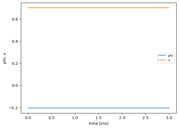

┌ Warning: Component model allocates similar arrays to inputs!
└ @ NetworkDynamics ~/.julia/packages/NetworkDynamics/xQuH4/src/doctor.jl:169