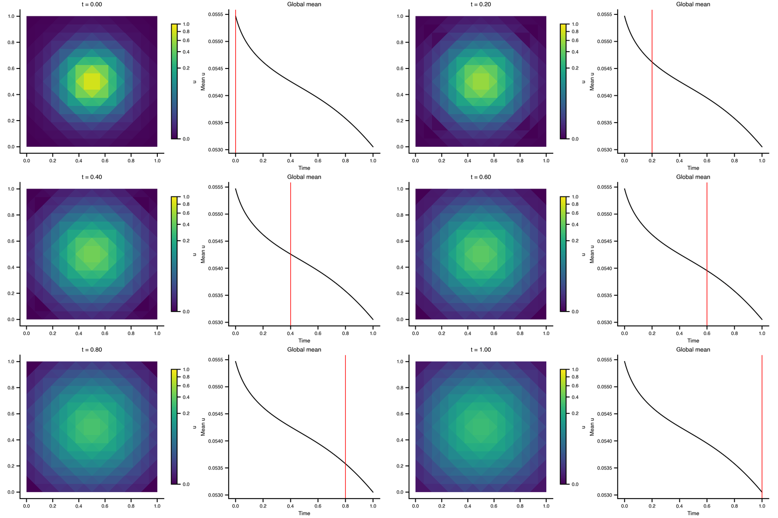
TVB-O integrates partial differential equations on a mesh with linear finite elements. The PDE backend generates a self-contained solver from a YAML experiment description, supporting triangle meshes (flat, or a curved surface in space, which is the cortical case) as well as tetrahedral meshes via scikit-fem, Dirichlet boundary conditions, declared events: as drives, and spatially varying coefficients.
The declared equation is the operator that runs. Each state variable’s equation.rhs is parsed into mass and stiffness blocks, so a system is lowered to
with one block row per state variable. Terms that are linear in the state go into \(A\) and are solved implicitly, which is unconditionally stable and lets the step size follow accuracy rather than a stability limit; anything else is evaluated at the current state each step. Because the constraint set and \(A\) are fixed, the sparse factorisation is computed once and every step is a triangular solve.
That covers rather more than diffusion:
You can write
Because
D * laplacian(u)
the classic heat equation
D * laplacian(u) - k * u
reaction terms become mass blocks
a system of several state_variables
one block row each, so second-order-in-time systems (waves) work
div(c * grad(u)) with per-vertex c
weighted stiffness assembly — a heterogeneous medium
a term naming an events: entry
the stimulus is substituted into the equation and evaluated each step
Time integration is Crank–Nicolson by default (second-order accurate and non-dissipative, which matters for waves: backward Euler damps oscillations artificially). Set method: implicit Euler for the first-order, strongly damping alternative.
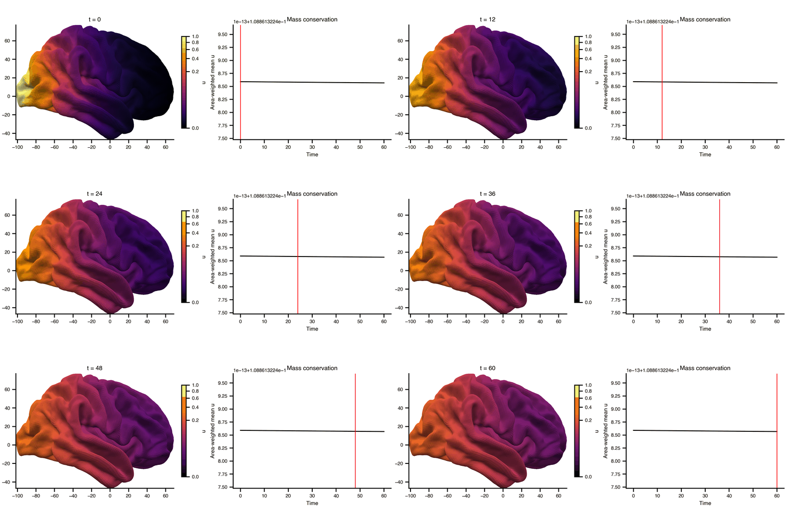
Diffusion on a cortical surface mesh (fsLR 32k), using the mesh_file attribute to reference an external GIFTI file directly. The cortical midthickness surface is a closed manifold (no boundary), so the Dirichlet BC has no effect and total mass is conserved, so the field spreads but doesn’t decay.
from matplotlib.colors import PowerNormfrom bsplot.surface import plot_surffrom bsplot.animate import animate_axesn_frames = ts2.data.shape[0]vmax2 =float(np.max(ts2.data))norm2 = PowerNorm(gamma=0.3, vmin=0, vmax=vmax2)fig2, (ax_surf, ax_ts) = plt.subplots(1, 2, figsize=(9, 4), layout="compressed")# Add a fixed colorbarimport matplotlib.cm as cmsm2 = cm.ScalarMappable(norm=norm2, cmap="inferno")fig2.colorbar(sm2, ax=ax_surf, label="u", shrink=0.8)# The conserved quantity is 1'Mu, so weight by the mass matrix the solver integrates# rather than by a second, hand-rolled notion of vertex area.from tvbo.data.mesh_fem import p1_massM_cortex = p1_mass(vertices, gi.darrays[1].data)vertex_areas = np.asarray(M_cortex.sum(axis=1)).ravel()global_mean = np.array([ (vertex_areas * np.asarray(ts2.data[t, 0, :])).sum() / vertex_areas.sum()for t inrange(n_frames)])def cortex_update(frame, ax, axis_idx, context): ax.clear()if axis_idx ==0: overlay = np.asarray(context["ts"].data[frame, 0, :]) plot_surf( context["gii"], overlay=overlay, hemi="rh", view="lateral", ax=ax, cmap="inferno", norm=context["norm"], ) ax.set_title(f"t = {context['ts'].time[frame]:.0f}")return []else: ax.plot(context["ts"].time, context["mean"], color="black") ax.axvline(context["ts"].time[frame], color="red", lw=1) ax.set_xlabel("Time") ax.set_ylabel("Area-weighted mean u") ax.set_title("Mass conservation")return []ctx = {"ts": ts2, "gii": gi, "norm": norm2, "mean": global_mean}anim2 = animate_axes(fig2, [ax_surf, ax_ts], n_frames=n_frames, update_fn=cortex_update, context=ctx, interval=200)anim2.save("_output/pde_cortex.gif", writer="pillow", fps=6)plt.close()
Cortical surface diffusion
Example 3: A damped wave equation with a heterogeneous medium
A second-order-in-time system, written as two first-order state variables, with a spatially varying propagation scale. This is the neural-field form used by geometric eigenmode models [1], generalised: those fit a single \(r_s\) for the whole cortex, which the modal route requires. Vary \(r_s\) in space and the operator stops being diagonal in the eigenbasis, so only a field formulation reaches this regime.
gamma =2.0exp_wave = {'label': 'Damped wave with heterogeneous propagation scale','field_dynamics': {'label': 'Damped wave','mesh': {'label': 'unit_square', 'element_type': 'triangle', 'mesh_file': mesh_path},# A parameter with no scalar value is a PER-VERTEX field. Give it a `producer:` and# the run needs no caller at all; passed to build() here so the sweep below can vary it.'parameters': {'g': {'name': 'g', 'value': gamma}, 'rsq': {'name': 'rsq', 'value': None}},'state_variables': [ {'name': 'phi', 'label': 'phi', 'initial_value': 1.0,'equation': {'lhs': 'phi_t', 'rhs': 'w'}}, {'name': 'w', 'label': 'w', 'initial_value': 0.0,'equation': {'lhs': 'w_t', 'rhs': 'g**2 * (-(2/g)*w - phi + div(rsq * grad(phi)))'}}, ],'solver': {'label': 'CN', 'discretization': 'FEM', 'method': 'crank-nicolson', 'dt': 0.005}, },'integration': {'duration': 2.0},}yaml_path3 = os.path.join(tmpdir, 'pde_wave.yaml')withopen(yaml_path3, 'w') as f: yaml.dump(exp_wave, f)exp3 = SimulationExperiment.from_file(yaml_path3)ns3 = exp3.execute('pde')print("per-vertex fields this system needs:", ns3['meta']['requires_fields'])# Fast propagation on the left half, slow on the rightxs = MeshTri.init_symmetric().refined(3).p[0]solve3, _, meta3 = ns3['build'](fields={'rsq': np.where(xs <0.5, 0.05, 0.005)})_, U3 = solve3(steps=400, save_timeseries=True)print(f"states: {meta3['variables']}, U shape {U3.shape}")
per-vertex fields this system needs: ['rsq']
states: ['phi', 'w'], U shape (401, 2, 145)
For the spatially uniform mode the Laplacian vanishes and the system is exactly critically damped, \(\phi = \phi_0(1+\gamma t)e^{-\gamma t}\), which is how the backend is verified:
t3 = np.arange(U3.shape[0]) *0.005analytic = (1+ gamma * t3) * np.exp(-gamma * t3)print(f"max deviation from the analytic envelope: {np.abs(U3[:, 0, :].mean(axis=1) - analytic).max():.2e}")
max deviation from the analytic envelope: 3.84e-06
Example 4: A brain wave equation, and the ODE system it becomes
Geometric eigenmode models of cortex [1] pose a damped wave equation on the cortical surface and then never integrate it. They expand the field in the eigenbasis of the Laplace–Beltrami operator, \(\Delta\psi_k = -\lambda_k\psi_k\), which turns the field equation into one damped oscillator per mode,
and integrate a few hundred of those instead. With constant coefficients this is an exact reformulation of the PDE, not an approximation of it, so the only error is the one introduced by stopping the sum. Having both routes in one framework is what turns that from a claim into a measurement.
The demonstration needs a closed curved surface, because that is the cortical case: no boundary anywhere, so a Dirichlet condition would constrain nothing.
import numpy as npfrom scipy.linalg import eighdef icosphere(subdivisions, radius):"""A closed triangulated sphere, refined by splitting every triangle in four.""" t = (1+5**0.5) /2 v = np.array([[-1,t,0],[1,t,0],[-1,-t,0],[1,-t,0],[0,-1,t],[0,1,t], [0,-1,-t],[0,1,-t],[t,0,-1],[t,0,1],[-t,0,-1],[-t,0,1]], float) f = np.array([[0,11,5],[0,5,1],[0,1,7],[0,7,10],[0,10,11],[1,5,9],[5,11,4], [11,10,2],[10,7,6],[7,1,8],[3,9,4],[3,4,2],[3,2,6],[3,6,8], [3,8,9],[4,9,5],[2,4,11],[6,2,10],[8,6,7],[9,8,1]])for _ inrange(subdivisions): mid, split, pts = {}, [], list(v)def midpoint(a, b): key = (min(a, b), max(a, b))if key notin mid: mid[key] =len(pts); pts.append((np.asarray(pts[a]) + pts[b]) /2)return mid[key]for a, b, c in f: ab, bc, ca = midpoint(a, b), midpoint(b, c), midpoint(c, a) split += [[a,ab,ca],[b,bc,ab],[c,ca,bc],[ab,bc,ca]] v, f = np.array(pts), np.array(split)return radius * v / np.linalg.norm(v, axis=1, keepdims=True), fvertices, faces = icosphere(3, 50.0) # mm, roughly a hemisphere's scalemeshio.Mesh(points=vertices, cells=[('triangle', faces)]).write( os.path.join(tmpdir, 'sphere.msh'))print(f"{len(vertices)} vertices, {len(faces)} triangles")
642 vertices, 1280 triangles
The equation is [1]’s, at their fitted parameters, driven by a 1 ms pulse declared as an events: entry. The backend substitutes it into the equation that names it:
Now the same system as modal ODEs. Solving \(K\psi = \lambda M\psi\) mass-orthonormally gives the discrete eigenbasis; each mode is stepped with the scheme the field solver uses, and the stimulus enters through its own projection \(\psi^\top M q\):
The last row is the point: with the complete basis the two agree to round-off, so the reformulation is exact and every row above it is pure truncation. That is what licenses reading a mode-truncated model’s residual as a statement about mode count rather than about the solver.
The sphere keeps the page fast, but nothing here changes at brain scale. On the full fsLR-32k left midthickness, at 32,492 vertices and 64,984 degrees of freedom for this two-variable system, assembling \(M\) and \(K\) takes 0.07 s, the sparse factorisation 8.4 s, and each subsequent step is a triangular solve at roughly 76 ms, in about 3 GiB. The factorisation cost is paid once because \(\Delta t\) and the operator are both fixed; changing either invalidates it.
Numerical details
The FEM update assembles mass (\(M\)) and stiffness (\(K\)) matrices over linear elements, builds the block operator \(A\) from the declared equations, and solves at each step
with \(\theta = \tfrac12\) for Crank–Nicolson and \(\theta = 1\) for implicit Euler. A term a * laplacian(u) contributes \(-aK\) (the weak form of the Laplacian is \(-\!\int\!\nabla u\cdot\nabla v\)), a term a * u contributes \(aM\), and div(c*grad(u)) contributes the weighted stiffness \(-\!\int\! c\,\nabla u\cdot\nabla v\).
meta carries the assembled mass_matrix, stiffness_matrix and operator, so a conservation law can be checked directly. Note that the conserved quantity of pure diffusion is \(\mathbf{1}^\top M\mathbf{u}\), not the nodal sum.
Triangles are assembled in closed form rather than through a FEM library, which is what makes a cortical mesh usable: it is a 2-manifold carrying three coordinates, and a general-purpose assembler expects the element and coordinate dimensions to agree. The P1 gradients on a surface triangle are tangential and known analytically, so the surface case is exact, and the stiffness matrix it produces is the familiar cotangent operator. Tetrahedra go through scikit-fem.
Surface operators carry the surface metric
A general-purpose assembler handed a curved triangle mesh does not necessarily refuse it. It may quietly discretise the mesh’s projection onto a coordinate plane, which runs, looks right, and answers a different question. On fsLR-32k that projection has an area of 33,070 mm² against the surface’s true 69,589 mm². The operators here are invariant under rotation and translation of the mesh, and tests/test_mesh_fem.py pins that against both scikit-fem (where the two agree, in the plane) and the analytic sphere spectrum (where only the surface form applies).
Not yet supported
c(x) * laplacian(u) is refused rather than approximated: its weak form requires \(\nabla c\) and is not self-adjoint. Write it in divergence form, div(c*grad(u)), which is conservative and symmetric. Neumann, Robin and Periodic boundary conditions are schema-only and raise if declared, rather than being silently dropped. Declared noise and coupling to a node-level dynamics: block are not lowered onto the field.
The explicit remainder \(\mathbf{f}\) is evaluated at the start of the step, so a system with a nonlinear or time-dependent term is first-order in time even under Crank–Nicolson. The linear part keeps its second order, and it is the linear part that sets stability.
Mesh Support
The Mesh class supports two ways to reference mesh geometry:
Attribute
Description
mesh_file
Path to external mesh file (GIFTI, VTK, MSH, FreeSurfer, etc.)
mesh_format
Explicit format override (gifti, freesurfer, meshio). Auto-detected from extension if omitted
dataLocation
Legacy attribute — still works, supports prefix syntax (gifti:path/to/file.gii)
Supported mesh formats:
Meshes are read by tvbo.data.mesh_io.read_mesh, the same reader the rest of TVB-O uses, so a surface behaves identically wherever it appears:
Format
Extensions
Loader
GIFTI
.gii, .surf.gii
nibabel
FreeSurfer
.pial, .white, .inflated, .sphere
nibabel
VTK
.vtk
parsed directly, including the ASCII PolyData form brain-surface templates ship in — which meshio refuses
Gmsh, VTU, OBJ, PLY
.msh, .vtu, .obj, .ply
meshio
Generated Code
The PDE backend generates a self-contained solver from the YAML specification:
code = exp.render_code("pde")print(code[:500])
The generated module contains:
Function
Purpose
_discretise()
Read the mesh and assemble the P1 operators its element type supports
build(fields=...)
Assemble the block operator and factor it once; fields supplies any per-vertex coefficient that did not declare its own provenance
solve_pde()
Crank–Nicolson / implicit Euler timestepping with optional source terms
visualize()
Matplotlib field plot, in the plane or on the surface
Schema Classes
Class
Purpose
PDE
Top-level PDE problem definition
SpatialDomain
Coordinate space and geometry
Mesh
Triangle/tetrahedron element mesh with mesh_file/mesh_format