TVB Monitor Round-Trip

Observation models — from YAML definition to TVB monitors and back, with TVB projection network visualization

TVB uses monitors to define what a simulation records — raw state variables, temporal averages, BOLD fMRI via hemodynamic response, or scalp EEG/MEG via lead-field projection. TVBO stores each monitor as a framework-agnostic Observation YAML that captures the full signal processing pipeline, then converts to any backend on demand.

import numpy as np
import matplotlib.pyplot as plt
from tvbo import Observation, Network

1. Observation Model Overview

Every observation model lives in tvbo/database/observation_models/ as a self-describing YAML file. Each defines:

• name / label — identifier and human-readable name
• class_reference — maps to a specific TVB monitor class
• period — sampling interval in ms
• pipeline — ordered signal processing steps (gain projection, HRF convolution, etc.)
• data_source — optional link to a sensor network (for EEG/MEG/iEEG)
• parameters — physical constants (conductivity, permeability, TR, …)

print("Available observation models:")
for name in Observation.list_db():
    obs = Observation.from_db(name)
    label = obs.label or obs.name
    pipe = len(obs.pipeline or [])
    ds = "sensor network" if obs.data_source else "—"
    print(f"  {str(obs.name):40s}  pipeline={pipe}  data_source={ds}")

Available observation models:
  AfferentCoupling                          pipeline=0  data_source=—
  AfferentCouplingTemporalAverage           pipeline=1  data_source=—
  BOLD_DoubleExponential                    pipeline=4  data_source=—
  BOLD_Gamma                                pipeline=4  data_source=—
  BOLD_MixtureOfGammas                      pipeline=4  data_source=—
  BOLD_RegionROI                            pipeline=6  data_source=—
  BOLD_TVB                                  pipeline=5  data_source=—
  EEG                                       pipeline=3  data_source=sensor network
  FunctionalConnectivity                    pipeline=4  data_source=—
  GlobalAverage                             pipeline=1  data_source=—
  MEG                                       pipeline=3  data_source=sensor network
  Raw                                       pipeline=0  data_source=—
  SpatialAverage                            pipeline=1  data_source=—
  SubSample                                 pipeline=1  data_source=—
  TemporalAverage                           pipeline=1  data_source=—
  iEEG                                      pipeline=3  data_source=sensor network

The models fall into four categories:

Category	Models	Key Feature
Basic	Raw, SubSample, TemporalAverage, GlobalAverage, SpatialAverage	Temporal/spatial reduction only
Projection	EEG, MEG, iEEG	Lead-field gain matrix + sensor network
Hemodynamic	BOLD (4 HRF variants), BoldRegionROI	HRF convolution + Volterra transform
Coupling	AfferentCoupling, AfferentCouplingTemporalAverage	Records coupling input, not state

2. Basic Monitors

Basic monitors apply simple temporal or spatial transformations to the raw simulation state. They require no external data.

obs_raw = Observation.from_db("raw")
print(f"{obs_raw.name}: {obs_raw.description}")
print(f"  Pipeline steps: {len(obs_raw.pipeline or [])}")
print(f"  TVB class: {obs_raw.class_reference.name}")

Raw: Records all state variables at every integration step without any transformation. Identity passthrough of the full simulation state.
  Pipeline steps: 0
  TVB class: Raw

obs_ta = Observation.from_db("temporal_average")
print(f"{obs_ta.name}: {obs_ta.label}")
print(f"  Period: {obs_ta.period} ms")
print(f"  Pipeline: {[str(s.name) for s in obs_ta.pipeline]}")

TemporalAverage: Temporal Average
  Period: 0.9765625 ms
  Pipeline: ['temporal_average']

Convert to TVB

Each observation converts to its corresponding TVB monitor with a single function call:

from tvbo.adapters.tvb import to_tvb_monitor

mon_raw = to_tvb_monitor(obs_raw)
mon_ta = to_tvb_monitor(obs_ta)

print(f"Raw  → {type(mon_raw).__name__}")
print(f"TA   → {type(mon_ta).__name__}, period={mon_ta.period}")

Raw  → Raw
TA   → TemporalAverage, period=0.9765625

3. Projection Monitors — EEG, MEG, iEEG

Projection monitors transform source-level neural activity into sensor signals via a lead-field (gain) matrix. Each model links to a sensor network stored as a YAML + HDF5 pair in the tvbo database.

The forward model pipeline:

1. Compute gain — load precomputed lead-field or use analytic formula (Sarvas 1987)
2. Lead-field projection — multiply gain matrix with source activity
3. Post-processing — re-referencing (EEG) or noise addition (MEG, iEEG)

3.1 EEG

obs_eeg = Observation.from_db("eeg")
print(f"{obs_eeg.name}: {obs_eeg.label}")
print(f"  Imaging modality: {obs_eeg.imaging_modality}")
print(f"  Sensor network:   {obs_eeg.data_source.path}")
print(f"  Pipeline: {[str(s.name) for s in obs_eeg.pipeline]}")

# Parameters
for pname, p in obs_eeg.parameters.items():
    unit = getattr(p, 'unit', '') or ''
    val = getattr(p, 'value', '—') or '—'
    print(f"  {pname}: {val} {unit}")

EEG: Scalp EEG
  Imaging modality: EEG
  Sensor network:   acq-EEGBrainstorm65_sensors.yaml
  Pipeline: ['compute_gain', 'lead_field_projection', 'rereference']
  conductivity: 1.0 S_per_m
  reference_electrode: — 

# Load the sensor network from database
from tvbo import database_path
sensor_net = Network.from_file(
    database_path / "networks" / obs_eeg.data_source.path
)
gain = sensor_net.matrix("gain", format="dense")

print(f"Sensor network: {sensor_net.number_of_nodes} electrodes")
print(f"Gain matrix:    {gain.shape} (sensors × vertices)")
print(f"Gain range:     [{np.nanmin(gain):.2f}, {np.nanmax(gain):.2f}]")

Sensor network: 65 electrodes
Gain matrix:    (65, 16384) (sensors × vertices)
Gain range:     [-120.12, 253.93]

3.2 MEG

obs_meg = Observation.from_db("meg")
print(f"{obs_meg.name}: {obs_meg.label}")
print(f"  Sensor network: {obs_meg.data_source.path}")
print(f"  Pipeline: {[str(s.name) for s in obs_meg.pipeline]}")

meg_net = Network.from_file(
    database_path / "networks" / obs_meg.data_source.path
)
meg_gain = meg_net.matrix("gain", format="dense")
print(f"  {meg_net.number_of_nodes} sensors, gain {meg_gain.shape}")

MEG: MEG
  Sensor network: acq-MEGBrainstorm276_sensors.yaml
  Pipeline: ['compute_gain', 'lead_field_projection', 'add_noise']
  276 sensors, gain (276, 16384)

3.3 iEEG (SEEG)

obs_ieeg = Observation.from_db("ieeg")
print(f"{obs_ieeg.name}: {obs_ieeg.label}")
print(f"  Sensor network: {obs_ieeg.data_source.path}")
print(f"  Pipeline: {[str(s.name) for s in obs_ieeg.pipeline]}")

iEEG: Intracranial EEG (SEEG)
  Sensor network: acq-SEEG588_sensors.yaml
  Pipeline: ['compute_gain', 'lead_field_projection', 'add_noise']

Convert Projection Monitors to TVB

The adapter loads sensors, orientations (MEG), and gain matrices automatically from the linked sensor network:

mon_eeg = to_tvb_monitor(obs_eeg)
mon_meg = to_tvb_monitor(obs_meg)
mon_ieeg = to_tvb_monitor(obs_ieeg)

print(f"EEG  → {type(mon_eeg).__name__}")
print(f"  Sensors:    {type(mon_eeg.sensors).__name__} {mon_eeg.sensors.locations.shape}")
print(f"  Projection: {type(mon_eeg.projection).__name__} {mon_eeg.projection.projection_data.shape}")

print(f"MEG  → {type(mon_meg).__name__}")
print(f"  Sensors:    {type(mon_meg.sensors).__name__} {mon_meg.sensors.locations.shape}")
print(f"  Projection: {type(mon_meg.projection).__name__} {mon_meg.projection.projection_data.shape}")

print(f"iEEG → {type(mon_ieeg).__name__}")
print(f"  Sensors:    {type(mon_ieeg.sensors).__name__} {mon_ieeg.sensors.locations.shape}")

EEG  → EEG
  Sensors:    SensorsEEG (65, 3)
  Projection: ProjectionSurfaceEEG (65, 16384)
MEG  → MEG
  Sensors:    SensorsMEG (276, 3)
  Projection: ProjectionSurfaceMEG (276, 16384)
iEEG → iEEG
  Sensors:    SensorsInternal (588, 3)

4. Visualize TVB Projection Networks on TVB Surface

We now build sensor-to-region projection graphs directly from the TVB-default EEG/MEG/iEEG monitor data and render them on the TVB default cortical surface mesh.

import nibabel as nib
from bsplot.graph import create_network, plot_network_on_surface
from tvbo import database_path
from tvb.datatypes.connectivity import Connectivity
from tvb.datatypes.surfaces import CorticalSurface
from tvb.datatypes.region_mapping import RegionMapping

# TVB default region/surface data
conn = Connectivity.from_file()
conn.configure()

surf = CorticalSurface.from_file()
surf.configure()

rmap = RegionMapping.from_file()
rmap.connectivity = conn
rmap.surface = surf
rmap.configure()

region_labels = list(conn.region_labels)
region_centers = conn.centres
n_regions = len(region_labels)

# Build a Gifti surface from TVB default cortical mesh (no template/MNI surface)
tvb_surface_gifti = nib.gifti.GiftiImage()
tvb_surface_gifti.add_gifti_data_array(
    nib.gifti.GiftiDataArray(
        np.asarray(surf.vertices, dtype=np.float32),
        intent="NIFTI_INTENT_POINTSET",
    )
)
tvb_surface_gifti.add_gifti_data_array(
    nib.gifti.GiftiDataArray(
        np.asarray(surf.triangles, dtype=np.int32),
        intent="NIFTI_INTENT_TRIANGLE",
    )
)

print(f"TVB surface: {surf.vertices.shape[0]} vertices, {surf.triangles.shape[0]} triangles")
print(f"TVB regions: {n_regions}")

TVB surface: 16384 vertices, 32760 triangles
TVB regions: 76

def _to_region_gain(gain_matrix, mapping, n_regions):
    gain_abs = np.abs(np.nan_to_num(gain_matrix, nan=0.0))

    # Already sensors × regions
    if gain_abs.shape[1] == n_regions:
        return gain_abs

    # Sensors × vertices -> aggregate using region mapping
    if gain_abs.shape[1] == len(mapping):
        out = np.zeros((gain_abs.shape[0], n_regions), dtype=float)
        for r in range(n_regions):
            mask = mapping == r
            if mask.any():
                out[:, r] = gain_abs[:, mask].mean(axis=1)
        return out

    raise ValueError(
        f"Unsupported gain shape {gain_abs.shape}; expected (*, {n_regions}) "
        f"or (*, {len(mapping)})"
    )


def _build_projection_graph(obs_name, layer_name, threshold_percentile=97):
    obs = Observation.from_db(obs_name)
    net = Network.from_file(database_path / "networks" / obs.data_source.path)

    sensor_labels = [str(n.label) for n in net.nodes]
    sensor_positions = np.asarray(
        [[n.position.x, n.position.y, n.position.z] for n in net.nodes],
        dtype=float,
    )
    n_sensors = len(sensor_labels)

    gain = net.matrix("gain", format="dense")
    if gain is None:
        return None, None  # No stored gain matrix (e.g. SEEG)

    region_gain = _to_region_gain(gain, rmap.array_data, n_regions)

    centers = {}
    for i, lbl in enumerate(region_labels):
        centers[f"R:{lbl}"] = tuple(region_centers[i])
    for i, lbl in enumerate(sensor_labels):
        centers[f"S:{lbl}"] = tuple(sensor_positions[i])

    combined = np.zeros((n_regions + n_sensors, n_regions + n_sensors), dtype=float)
    for i in range(n_sensors):
        for j in range(n_regions):
            combined[n_regions + i, j] = region_gain[i, j]

    labels = [f"R:{x}" for x in region_labels] + [f"S:{x}" for x in sensor_labels]
    graph = create_network(
        centers,
        {layer_name: combined},
        labels=labels,
        threshold_percentile=threshold_percentile,
        directed=True,
        edge_data_key="gain",
    )

    for node in graph.nodes():
        graph.nodes[node]["color"] = "gold" if node.startswith("R:") else "crimson"

    return graph, region_gain

candidates = {
    "EEG": ("eeg", "eeg_projection"),
    "MEG": ("meg", "meg_projection"),
    "iEEG/SEEG": ("ieeg", "ieeg_projection"),
}

graphs = {}
for name, (obs_name, layer) in candidates.items():
    result = _build_projection_graph(obs_name, layer)
    if result[0] is None:
        print(f"{name:10s} — no stored gain matrix, skipped")
    else:
        g, rg = result
        graphs[name] = (g, rg)
        print(
            f"{name:10s} nodes={g.number_of_nodes():3d} edges={g.number_of_edges():5d} "
            f"gain=[{rg.min():.2e}, {rg.max():.2e}]"
        )

EEG        nodes=141 edges=  144 gain=[0.00e+00, 5.49e+01]
MEG        nodes=352 edges=  566 gain=[0.00e+00, 9.42e-06]
iEEG/SEEG  — no stored gain matrix, skipped

n_plots = len(graphs)
fig, axes = plt.subplots(1, n_plots, figsize=(5 * n_plots, 5))
if n_plots == 1:
    axes = [axes]

for ax, (title, (graph, _)) in zip(axes, graphs.items()):
    plot_network_on_surface(
        graph,
        ax=ax,
        template=tvb_surface_gifti,
        hemi="lh",
        view="top",
        node_radius=1.4,
        node_color="auto",
        edge_radius=0.003,
        edge_color="auto",
        edge_data_key="gain",
        edge_cmap="viridis",
        edge_scale={"gain": 10, "mode": "quantile"},
        surface_alpha=0.12,
    )
    ax.set_title(f"{title} ({graph.number_of_edges()} edges)")

plt.tight_layout()
plt.show()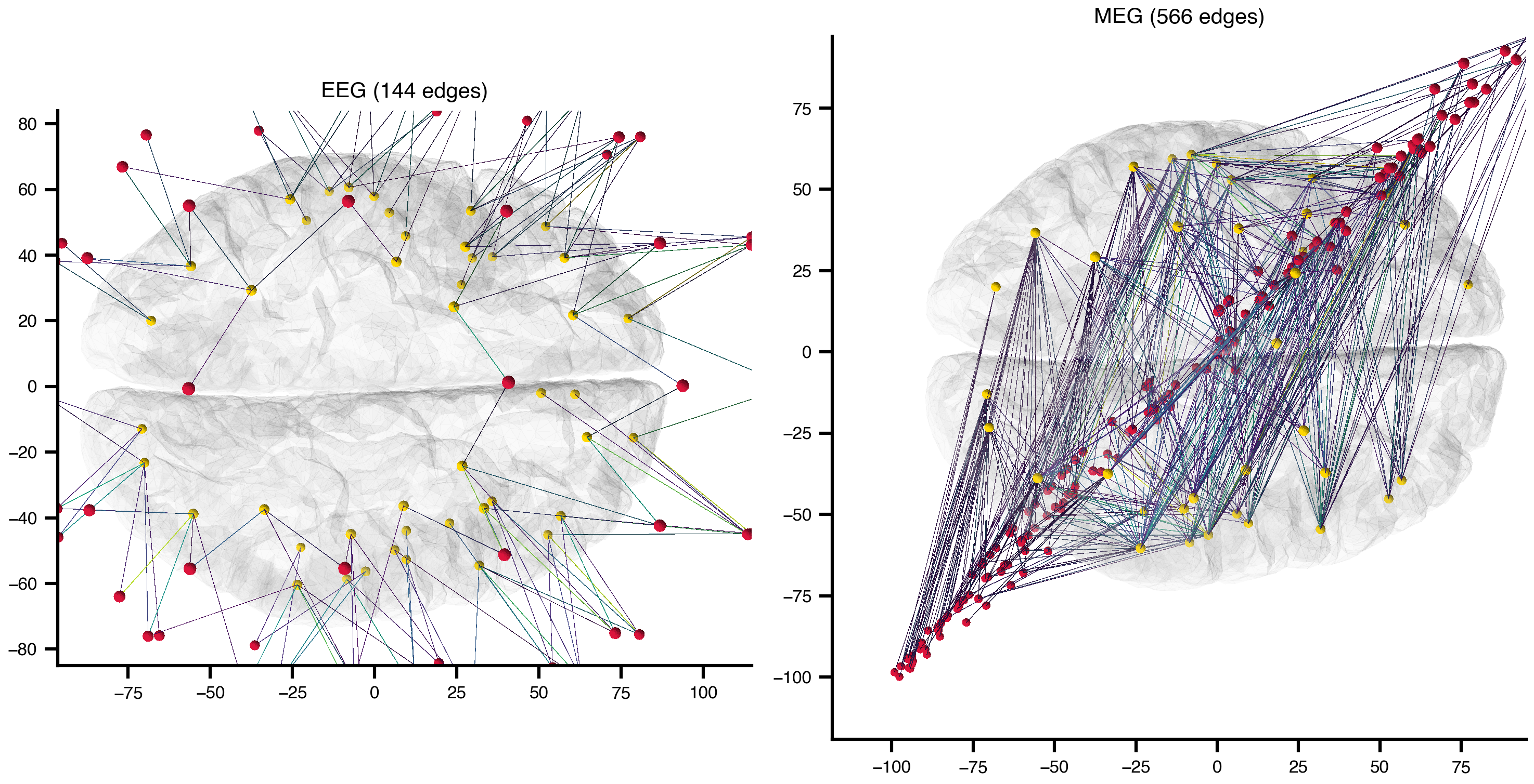

Figure 1: TVB default projection networks on the TVB default cortical surface.

5. Hemodynamic Monitors (BOLD)

BOLD monitors simulate the fMRI signal by convolving neural activity with a hemodynamic response function (HRF), followed by temporal subsampling at the repetition time (TR).

The pipeline:

1. Temporal averaging — interim downsampling before convolution
2. HRF generation — compute the kernel (Volterra, Gamma, DoubleExponential, MixtureOfGammas)
3. Convolution — scipy.signal.fftconvolve with HRF kernel
4. Subsampling — downsample to TR
5. Volterra transform — nonlinear signal transformation (some variants)

obs_bold = Observation.from_db("bold_tvb")
print(f"{obs_bold.name}: {obs_bold.label}")
print(f"  HRF kernel: {obs_bold.class_reference.constructor_args[0].value}")
print(f"  Pipeline: {[str(s.name) for s in obs_bold.pipeline]}")

# Show HRF equation
hrf_step = [s for s in obs_bold.pipeline if str(s.name) == 'hemodynamic_response'][0]
print(f"  HRF equation: {hrf_step.equation.rhs}")
for pname, p in hrf_step.equation.parameters.items():
    print(f"    {pname} = {p.value} {getattr(p, 'unit', '')}")

BOLD_TVB: BOLD (First Order Volterra)
  HRF kernel: FirstOrderVolterra
  Pipeline: ['temporal_average_interim', 'hemodynamic_response', 'convolve', 'subsample_to_period', 'volterra_transform']
  HRF equation: 1/3 * exp(-0.5*(t / tau_s)) * sin(sqrt(1/tau_f - 1/(4*tau_s**2)) * t) / sqrt(1/tau_f - 1/(4*tau_s**2))
    tau_f = 0.4 s
    tau_s = 0.8 s

mon_bold = to_tvb_monitor(obs_bold)
print(f"BOLD → {type(mon_bold).__name__}")
print(f"  HRF: {type(mon_bold.hrf_kernel).__name__}")
print(f"  Period: {mon_bold.period} ms")

# Available BOLD variants
bold_variants = [n for n in Observation.list_db() if 'bold' in n.lower()]
for name in bold_variants:
    obs = Observation.from_db(name)
    cr = obs.class_reference
    hrf = next((a.value for a in (cr.constructor_args or []) if str(a.name) == 'hrf_kernel'), '—')
    print(f"  {str(obs.name):30s}  HRF={hrf}")

BOLD → Bold
  HRF: FirstOrderVolterra
  Period: 2000.0 ms
  BOLD_DoubleExponential          HRF=DoubleExponential
  BOLD_Gamma                      HRF=Gamma
  BOLD_MixtureOfGammas            HRF=MixtureOfGammas
  BOLD_RegionROI                  HRF=FirstOrderVolterra
  BOLD_TVB                        HRF=FirstOrderVolterra

6. Coupling Monitors

Coupling monitors record the afferent (incoming) coupling term at each node — the network input that drives the dynamics, rather than the model state itself. Useful for analysing effective connectivity.

obs_ac = Observation.from_db("afferent_coupling")
print(f"{obs_ac.name}: {obs_ac.label}")
print(f"  Source: {obs_ac.source}")
print(f"  Pipeline steps: {len(obs_ac.pipeline or [])}")

mon_ac = to_tvb_monitor(obs_ac)
print(f"  → {type(mon_ac).__name__}")

AfferentCoupling: Afferent Coupling Recording
  Source: coupling
  Pipeline steps: 0
  → AfferentCoupling

7. Simulation Round-Trip: Numerical Verification

To verify that tvbo-generated TVB models are faithful to the original, we compare simulations run with the TVB-native Generic2dOscillator against the tvbo-generated equivalent. Both use identical connectivity, coupling, integrator, and initial conditions. Results are wrapped using ExperimentResult.from_tvb() for consistent access.

from tvbo import Dynamics, ExperimentResult
from tvb.simulator.lab import simulator, models, coupling, integrators, monitors

# Shared setup
sim_length = 100.0  # ms
seed = 42

# --- TVB Native ---
m1 = models.Generic2dOscillator()
m1.variables_of_interest = ('V', 'W')
sim1 = simulator.Simulator(
    model=m1,
    coupling=coupling.Linear(a=np.array([0.0126])),
    integrator=integrators.HeunDeterministic(dt=0.1),
    connectivity=conn,
    monitors=[monitors.Raw()],
    simulation_length=sim_length,
)
np.random.seed(seed)
sim1.configure()
result_native = ExperimentResult.from_tvb(sim1)

# --- tvbo Generated ---
m = Dynamics.from_db('Generic2dOscillator')
code = m.render_code('tvb')
ns = {}
exec(code, ns)
m2 = ns['Generic2dOscillator']()
sim2 = simulator.Simulator(
    model=m2,
    coupling=coupling.Linear(a=np.array([0.0126])),
    integrator=integrators.HeunDeterministic(dt=0.1),
    connectivity=conn,
    monitors=[monitors.Raw()],
    simulation_length=sim_length,
)
np.random.seed(seed)
sim2.configure()
result_tvbo = ExperimentResult.from_tvb(sim2)

print(f"TVB native cvar:     {sim1.model.cvar}")
print(f"tvbo-generated cvar: {sim2.model.cvar}")
print(f"Output shape: {result_native.integration.data.shape}")

diff = np.abs(result_native.integration.data - result_tvbo.integration.data).max()
print(f"Max absolute diff:   {diff:.2e}")
print(f"Numerically equal:   {np.allclose(result_native.integration.data, result_tvbo.integration.data, atol=1e-10)}")

TVB native cvar:     [0]
tvbo-generated cvar: [0]
Output shape: (1000, 2, 76, 1)
Max absolute diff:   3.55e-15
Numerically equal:   True

ts_native = result_native.integration
ts_tvbo = result_tvbo.integration

node = 0
fig, (ax1, ax2) = plt.subplots(2, 1, figsize=(10, 4), sharex=True, height_ratios=[3, 1])

ts_native.get_subspace_by_index([node]).plot(ax=ax1, label="TVB native", linewidth=1.5)
ts_tvbo.get_subspace_by_index([node]).plot(ax=ax1, label="tvbo-generated", linestyle="--", linewidth=1.5)
ax1.legend()
ax1.set_title(f"Region {node}: {conn.region_labels[node]}")

diff_trace = np.abs(ts_native.data.isel(variable=0, node=node, mode=0) - ts_tvbo.data.isel(variable=0, node=node, mode=0)) + 1e-20
ax2.semilogy(ts_native.time, diff_trace, color="k", lw=0.8)
ax2.set_ylabel("|diff|")
ax2.set_xlabel("Time (ms)")

plt.tight_layout()
plt.show()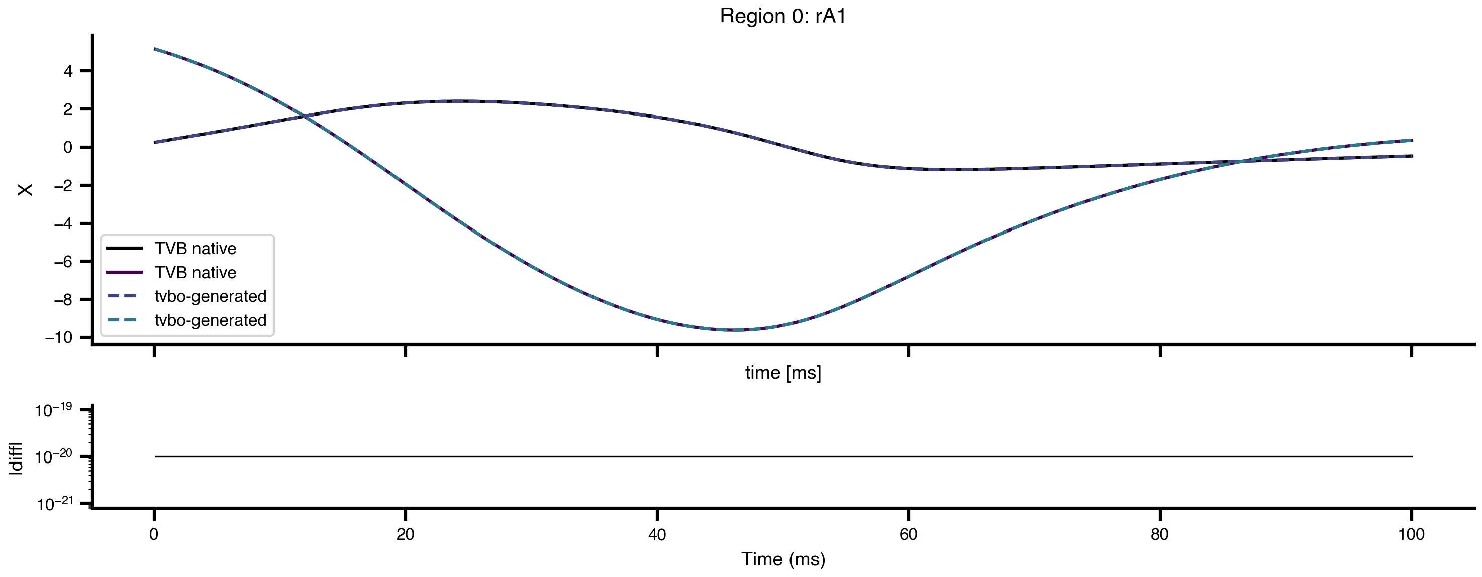

Figure 2: Simulation roundtrip: TVB native vs tvbo-generated Generic2dOscillator. Top: raw V traces for one region. Bottom: absolute difference (machine-epsilon level).

Code Generation API

Each observation model can also render its TVB monitor code directly:

obs_eeg_rt = Observation.from_db("eeg")
print(obs_eeg_rt.render_code("tvb"))

import abc
import numpy
from tvb.simulator.monitors import Monitor
from tvb.simulator.monitors import Projection
from tvb.basic.neotraits.api import Float, NArray, Attr
from tvb.simulator.backend.ref import ReferenceBackend
from tvb.datatypes.sensors import SensorsEEG
from tvb.datatypes.projections import ProjectionSurfaceEEG
from tvb.simulator import noise
from tvb.datatypes.region_mapping import RegionMapping
from tvb.simulator.common import numpy_add_at


class EEG(Projection):
    """Lead-field projection monitor (EEG)."""

    period = Float(default=0.9765625)
    sigma = Float(default=1.0)
    sensors = Attr(SensorsEEG, required=True)
    projection = Attr(ProjectionSurfaceEEG, default=None)
    reference = Attr(str, required=False, default=None)

    def analytic(self, loc, ori):
        """Sarvas 1987 single-sphere approximation (Eq. 12)."""
        r_0, Q = loc, ori
        centre = numpy.mean(r_0, axis=0)[numpy.newaxis, :]
        radius = 1.05125 * max(numpy.sqrt(numpy.sum((r_0 - centre) ** 2, axis=1)))
        sen_loc = self.sensors.locations.copy()
        sen_dis = numpy.sqrt(numpy.sum(sen_loc**2, axis=1))
        sen_loc = sen_loc / sen_dis[:, numpy.newaxis] * radius + centre
        V_r = numpy.zeros((sen_loc.shape[0], r_0.shape[0]))
        for k in range(sen_loc.shape[0]):
            a = sen_loc[k, :] - r_0
            na = numpy.sqrt(numpy.sum(a**2, axis=1))[:, numpy.newaxis]
            V_r[k, :] = numpy.sum(Q * (a / na**3), axis=1) / (
                4.0 * numpy.pi * self.sigma
            )
        return V_r

    def config_for_sim(self, simulator):
        super(EEG, self).config_for_sim(simulator)
        n_sensors = self.sensors.number_of_sensors
        self._ref_vec = numpy.zeros((n_sensors,))
        if self.reference:
            if self.reference.lower() != "average":
                idx = self.sensors.labels.tolist().index(self.reference)
                self._ref_vec[idx] = 1.0
            else:
                self._ref_vec[:] = 1.0 / n_sensors
        self._ref_vec_mask = numpy.isfinite(self.gain).all(axis=1)
        self._ref_vec = self._ref_vec[self._ref_vec_mask]

    def sample(self, step, state):
        maybe = super(EEG, self).sample(step, state)
        if maybe is not None:
            time, sample = maybe
            sample -= self._ref_vec.dot(sample[:, self._ref_vec_mask])[:, numpy.newaxis]
            return time, sample.reshape((self.voi.size, -1, 1))


monitors = [
    EEG(sensors=SensorsEEG.from_file(), projection=ProjectionSurfaceEEG.from_file()),
]

# Execute returns a configured TVB monitor object
mon = obs_eeg_rt.execute("tvb")
print(f"Returned: {type(mon).__name__}")
if hasattr(mon, 'sensors') and mon.sensors is not None:
    print(f"  Sensors: {mon.sensors.locations.shape}")

Returned: EEG
  Sensors: (65, 3)

8. Monitor Round-Trip: tvbo → TVB → verify

The adapter can convert every observation type to its corresponding TVB monitor and back:

from tvbo.adapters.tvb import to_tvb_monitor

for name in ["raw", "eeg", "bold_tvb", "temporal_average"]:
    obs = Observation.from_db(name)
    mon = to_tvb_monitor(obs)
    print(f"{str(obs.name):20s} → {type(mon).__name__:30s}", end="")

    if hasattr(mon, 'sensors') and mon.sensors is not None:
        print(f"  sensors={mon.sensors.locations.shape}", end="")
    if hasattr(mon, 'projection') and mon.projection is not None:
        print(f"  gain={mon.projection.projection_data.shape}", end="")
    if hasattr(mon, 'hrf_kernel') and mon.hrf_kernel is not None:
        print(f"  hrf={type(mon.hrf_kernel).__name__}", end="")
    print()

Raw                  → Raw                           
EEG                  → EEG                             sensors=(65, 3)  gain=(65, 16384)
BOLD_TVB             → Bold                            hrf=FirstOrderVolterra
TemporalAverage      → TemporalAverage               

Summary

Step	Method	What It Does
List	Observation.list_db()	Show all available observation models
Load	Observation.from_db("eeg")	Load observation from database by name
File	Observation.from_file("path.yaml")	Load from arbitrary YAML file
Export	to_tvb_monitor(obs)	Convert to configured TVB Monitor
Sensors	Network.from_file(database_path / "networks" / obs.data_source.path)	Load linked sensor network
Gain	sensor_net.matrix("gain", format="dense")	Access lead-field matrix

The observation model YAML captures the complete signal processing chain — from raw neural activity to the measured signal — in a framework-agnostic format that any backend can consume.