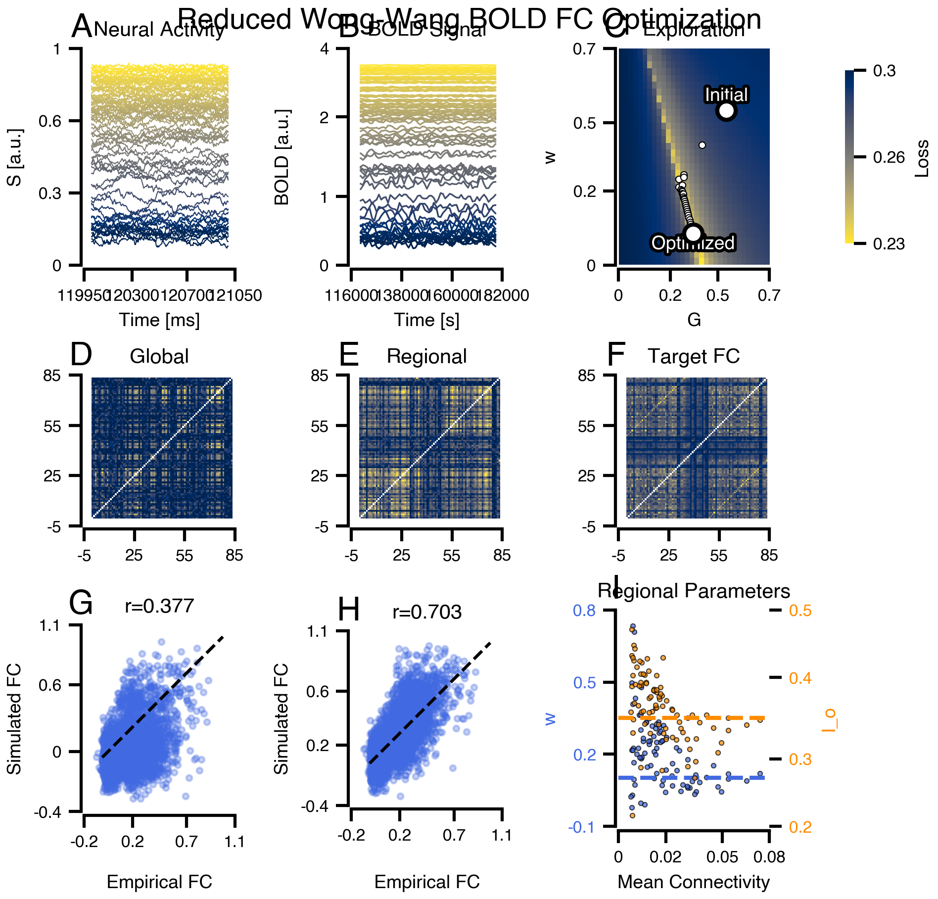
# | fig-cap: "**RWW BOLD FC Optimization.** (A) Neural activity. (B) BOLD signal. (C) Parameter landscape with trajectory. (D-F) FC matrices: target, global, regional. (G-H) FC scatter plots. (I-J) Fitted regional parameters."

import bsplot
from matplotlib.colors import Normalize
import matplotlib.pyplot as plt
import matplotlib.patheffects as path_effects
import jax.numpy as jnp
import numpy as np
from tvboptim.observations.observation import fc_corr

mosaic = """
AABBCC
DDEEFF
GGHHII
"""
fig, axes = plt.subplot_mosaic(mosaic, layout='compressed', figsize=(8, 6))
cmap = plt.cm.cividis

fc_target = results.integration.observations.empirical_fc

# A: Neural Activity
ax = axes["A"]
t_max = int(1000 / exp.integration.step_size)
data = np.asarray(results.integration.data[:t_max, 0, :])
norm = Normalize(vmin=data.mean(0).min(), vmax=data.mean(0).max())
for i in range(data.shape[1]):
    ax.plot(
        np.asarray(results.integration.time[:t_max]),
        data[:, i],
        color=cmap(norm(data.mean(0)[i])),
        lw=0.5,
    )
ax.set(xlabel="Time [ms]", ylabel="S [a.u.]", title="Neural Activity")

# B: BOLD Signal
ax = axes["B"]
bold = results.integration.observations.bold
data = np.asarray(bold.data[:60, 0, :])
norm = Normalize(vmin=data.mean(0).min(), vmax=data.mean(0).max())
for i in range(data.shape[1]):
    ax.plot(np.asarray(bold.time[:60]), data[:, i], color=cmap(norm(data.mean(0)[i])), lw=0.8)
ax.set(xlabel="Time [s]", ylabel="BOLD [a.u.]", title="BOLD Signal")

# C: Parameter Landscape with Trajectory
ax = axes["C"]
expl = results.exploration.parameter_landscape
# Labeled loss landscape: as_grid() is an xarray keyed by the dotted parameters,
# so orient it by name (order-independent) and read the coords straight off it.
loss = expl.as_grid().transpose("ReducedWongWang.w", "FastLinearCoupling.G")
w_vals, G_vals = loss["ReducedWongWang.w"].values, loss["FastLinearCoupling.G"].values
im = ax.imshow(
    loss.values,
    cmap="cividis_r",
    extent=[G_vals.min(), G_vals.max(), w_vals.min(), w_vals.max()],
    origin="lower",
    aspect="auto",
)
plt.colorbar(im, ax=ax, label="Loss", shrink=0.8)

# Initial & fitted points
for label, G, w, dy in [
    (
        "Initial",
        results.state.coupling.FastLinearCoupling.G,
        results.state.dynamics.w,
        0.03,
    ),
    (
        "Optimized",
        results.global_optimization.fitted_params.coupling.FastLinearCoupling.G.value,
        results.global_optimization.fitted_params.dynamics.w.value,
        -0.05,
    ),
]:
    ax.scatter(
        G, w, color="white", s=80, marker="o", edgecolors="k", linewidths=2, zorder=5
    )
    ax.annotate(
        label,
        (G, w),
        xytext=(G, w + dy),
        color="white",
        fontweight="bold",
        ha="center",
        path_effects=[path_effects.withStroke(linewidth=3, foreground="black")],
    )

# Trajectory
route = results.optimizations.global_optimization.state_trajectory
ax.scatter(
    [s.coupling.FastLinearCoupling.G.value for s in route],
    [s.dynamics.w.value for s in route],
    color="white",
    s=10,
    marker="o",
    edgecolors="k",
    linewidths=0.5,
    zorder=4,
)
ax.set(xlabel="G", ylabel="w", title="Exploration")

# D-F: FC Matrices
for key, fc, title in [
    ("D", np.array(results.optimizations.global_optimization.simulation.observations.fc), f"Global"),
    ("E", np.array(results.optimizations.regional_optimization.simulation.observations.fc), f"Regional"),
    ("F", fc_target, "Target FC"),
]:
    ax = axes[key]
    fc_plot = np.copy(fc)
    np.fill_diagonal(fc_plot, np.nan)
    ax.imshow(fc_plot, cmap="cividis", vmin=0, vmax=0.9)
    ax.set(xticks=[], yticks=[], title=title)

# G-H: Scatter Plots
triu = np.triu_indices_from(fc_target, k=1)
for key, fc, title in [
    ("G", results.optimizations.global_optimization.simulation.observations.fc, "Global Fit"),
    ("H", results.optimizations.regional_optimization.simulation.observations.fc, "Regional Fit"),
]:
    ax = axes[key]
    ax.scatter(fc_target[triu], np.array(fc)[triu], alpha=0.3, s=8, color="royalblue")
    ax.plot([0, 1], [0, 1], "k--", lw=1.5)
    ax.set(
        xlabel="Empirical FC",
        ylabel="Simulated FC",
        title=f"r={fc_corr(fc, fc_target):.3f}",
        aspect="equal",
    )

# I: Fitted Regional Parameters (dual y-axis)
mean_conn = exp.network.weights.mean(axis=1)
opt_g, opt_r = results.global_optimization, results.regional_optimization

ax1 = axes["I"]

ax2 = ax1.twinx()

# Left axis: w (blue)
ax1.scatter(
    mean_conn,
    opt_r.fitted_params.dynamics.w.value.flatten(),
    alpha=0.7,
    s=5,
    color="royalblue",
    edgecolors="k",
    lw=0.5,
    label="w (regional)",
)
ax1.axhline(
    opt_g.fitted_params.dynamics.w.value,
    color="royalblue",
    ls="--",
    lw=2,
    label=f"w (global): {float(opt_g.fitted_params.dynamics.w.value):.3f}",
)
ax1.set_xlabel("Mean Connectivity")
ax1.set_ylabel("w", color="royalblue")
ax1.tick_params(axis="y", labelcolor="royalblue")

# Right axis: I_o (orange)
ax2.scatter(
    mean_conn,
    opt_r.fitted_params.dynamics.I_o.value.flatten(),
    alpha=0.7,
    s=5,
    color="darkorange",
    edgecolors="k",
    lw=0.5,
    label="I_o (regional)",
)
ax2.axhline(
    opt_g.fitted_params.dynamics.I_o,
    color="darkorange",
    ls="--",
    lw=2,
    label=f"I_o (global): {float(opt_g.fitted_params.dynamics.I_o):.3f}",
)
ax2.set_ylabel("I_o", color="darkorange")
ax2.tick_params(axis="y", labelcolor="darkorange")

ax1.set_title("Regional Parameters")
# lines1, labels1 = ax1.get_legend_handles_labels()
# lines2, labels2 = ax2.get_legend_handles_labels()
# ax1.legend(lines1 + lines2, labels1 + labels2, loc="upper right", fontsize=8)

plt.suptitle(
    "Reduced Wong-Wang BOLD FC Optimization", fontsize=14, fontweight="bold", y=1
)
bsplot.style.format_fig(fig)
##