5. Hysteresis (Double Saddle-Node)

A small constant tilt added to the pitchfork unfolds it into a hysteresis curve with two saddle-node bifurcations:

\[ \dot x = a + x - x^3. \]

The bifurcation diagram in \((a, x)\) is the classic S-curve with two folds (vertical tangents) at \(a_{\pm} = \pm\,2/(3\sqrt 3) \approx \pm 0.385\), framing a bistable region in which the system has two coexisting stable states separated by an unstable middle branch. Reproduces Hysteresis.png.

from tvbo import Dynamics, Continuation, SimulationExperiment
import matplotlib.pyplot as plt
import numpy as np

HY_YAML = """
name: Hysteresis
description: Double saddle-node / hysteresis $\\dot x = a + x - x^3$.
parameters:
  a:
    name: a
    value: 0.0
state_variables:
  x:
    name: x
    domain: { lo: -2.0, hi: 2.0 }
    equation:
      lhs: Derivative(x, t)
      rhs: a + x - x**3
    initial_value: 1.0
"""

CONT_YAML = """
name: hy_in_a
dynamics: Hysteresis
free_parameters:
  - name: a
    domain: { lo: -2.0, hi: 2.0 }
max_steps: 600
ds: 0.005
bothside: true
"""

dyn = Dynamics.from_string(HY_YAML)
cont = Continuation.from_string(CONT_YAML)
exp = SimulationExperiment(dynamics=dyn, continuations=[cont])

BifurcationKit.jl

result_jl = exp.run("bifurcationkit.jl")
result_jl.continuations["hy_in_a"].plot(VOI="x")
plt.gca().set_xlim(-1, 1); plt.gca().set_ylim(-2, 2); plt.show()

Detected IPython. Loading juliacall extension. See https://juliapy.github.io/PythonCall.jl/stable/compat/#IPython
CT: 1.312985 seconds (3.31 M allocations: 165.801 MiB, 99.86% compilation time)
CT: 0.000496 seconds (10.02 k allocations: 416.578 KiB)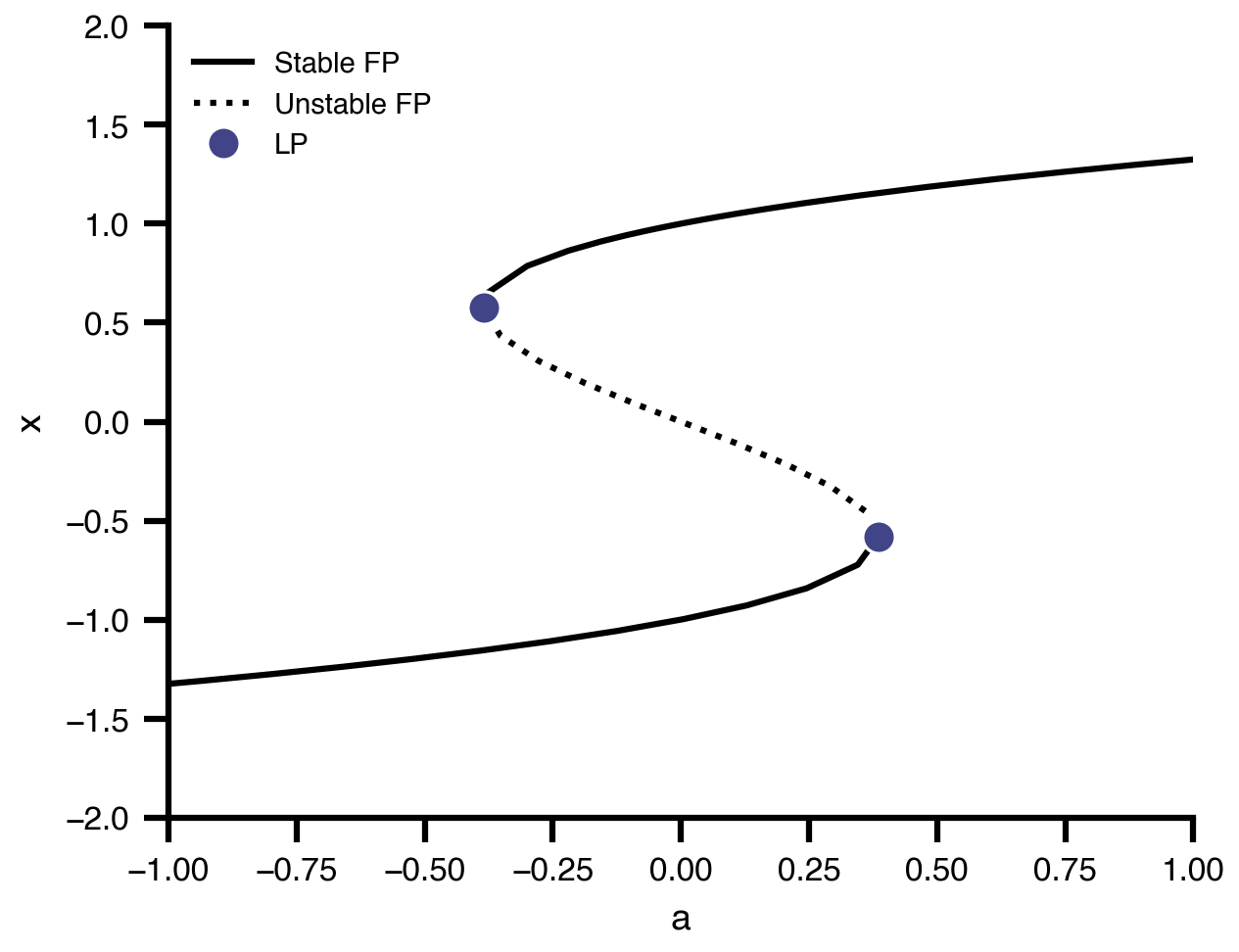

PyRates / PyCoBi

PyCoBi requires NDIM >= 2; the adapter raises a clear error for this 1-D system. Use auto-07p or bifurcationkit.jl instead.

try:
    result_py = exp.run("pyrates-bifurcation")
    result_py.continuations["hy_in_a"].plot(VOI="x")
except NotImplementedError as e:
    print(e)

Compilation Progress
--------------------
    (1) Translating the circuit template into a networkx graph representation...
        ...finished.
    (2) Preprocessing edge transmission operations...
        ...finished.
    (3) Parsing the model equations into a compute graph...
        ...finished.
    Model compilation was finished.
The 'pyrates-bifurcation' backend cannot continue the 1-D system 'Hysteresis' (state variables: ['x']). PyCoBi's summary builder requires NDIM >= 2 and raises KeyError('U(1)') for scalar ODEs. For 1-D systems use the 'auto-07p' or 'bifurcationkit.jl' backend instead.

AUTO-07p (NumCont)

Direct analogue of the standalone DoubleSaddleNode.py example. AUTO-07p time-integrates from the model defaults to land on the upper stable branch, then sweeps \(a\) in both directions so both saddle-nodes are picked up in a single merged diagram.

result_auto = exp.run("auto-07p")
result_auto.continuations["hy_in_a"].plot(VOI="x")
plt.gca().set_xlim(-1, 1); plt.gca().set_ylim(-2, 2); plt.show()

/opt/homebrew/bin/gfortran -arch arm64 -O -fopenmp -O -c /var/folders/ym/9kw1g21j1nd7kwfn8c0z3st40000gn/T/tvbo_numcont_Hysteresis_u5ns4xyw/model.f90 -o /var/folders/ym/9kw1g21j1nd7kwfn8c0z3st40000gn/T/tvbo_numcont_Hysteresis_u5ns4xyw/model.o
/opt/homebrew/bin/gfortran -arch arm64 -O -fopenmp -O /var/folders/ym/9kw1g21j1nd7kwfn8c0z3st40000gn/T/tvbo_numcont_Hysteresis_u5ns4xyw/model.o -o /var/folders/ym/9kw1g21j1nd7kwfn8c0z3st40000gn/T/tvbo_numcont_Hysteresis_u5ns4xyw/model.exe /Applications/auto-07p/lib/*.o
Starting /var/folders/ym/9kw1g21j1nd7kwfn8c0z3st40000gn/T/tvbo_numcont_Hysteresis_u5ns4xyw/model ...

ld: warning: duplicate -rpath '/Library/Developer/CommandLineTools/SDKs/MacOSX26.4.sdk/usr/lib' ignored


  BR    PT  TY  LAB       a          L2-NORM          x       
   1     1  EP    1   0.00000E+00   1.00000E+00   1.00000E+00
   1    10        2   8.70787E-02   1.04099E+00   1.04099E+00
   1    20        3   2.32804E-01   1.10069E+00   1.10069E+00
   1    30        4   4.15909E-01   1.16492E+00   1.16492E+00
   1    40        5   6.58325E-01   1.23770E+00   1.23770E+00
   1    50        6   1.01405E+00   1.32800E+00   1.32800E+00
   1    60        7   1.51549E+00   1.43413E+00   1.43413E+00
   1    67  EP    8   2.01998E+00   1.52473E+00   1.52473E+00

 Total Time    0.161E-02
/var/folders/ym/9kw1g21j1nd7kwfn8c0z3st40000gn/T/tvbo_numcont_Hysteresis_u5ns4xyw/model ... done
Starting /var/folders/ym/9kw1g21j1nd7kwfn8c0z3st40000gn/T/tvbo_numcont_Hysteresis_u5ns4xyw/model ...

  BR    PT  TY  LAB       a          L2-NORM          x       
   1     1  EP    1   0.00000E+00   1.00000E+00   1.00000E+00
   1    10        2  -8.48200E-02   9.54537E-01   9.54537E-01
   1    20        3  -1.79557E-01   8.93947E-01   8.93947E-01
   1    30        4  -2.66212E-01   8.22365E-01   8.22365E-01
   1    40        5  -3.37505E-01   7.35690E-01   7.35690E-01
   1    50        6  -3.79562E-01   6.32009E-01   6.32009E-01
   1    55  LP    7  -3.84900E-01   5.77340E-01   5.77340E-01
   1    60        8  -3.79655E-01   5.21411E-01   5.21411E-01
   1    70        9  -3.43618E-01   4.15189E-01   4.15189E-01
   1    80       10  -2.86232E-01   3.18560E-01   3.18560E-01
   1    90       11  -2.17471E-01   2.29569E-01   2.29569E-01
   1   100       12  -1.27124E-01   1.29285E-01   1.29285E-01
   1   110       13   1.47482E-01   1.50919E-01  -1.50919E-01
   1   116  LP   14   3.84900E-01   5.77358E-01  -5.77358E-01
   1   120       15   2.19388E-01   8.63709E-01  -8.63709E-01
   1   130       16  -5.57072E-01   1.20867E+00  -1.20867E+00
   1   140       17  -1.38732E+00   1.40881E+00  -1.40881E+00
   1   148  EP   18  -2.05965E+00   1.53134E+00  -1.53134E+00

 Total Time    0.207E-02
/var/folders/ym/9kw1g21j1nd7kwfn8c0z3st40000gn/T/tvbo_numcont_Hysteresis_u5ns4xyw/model ... done
Merge done
Saving to hy_in_a, hy_in_a, and hy_in_a ... done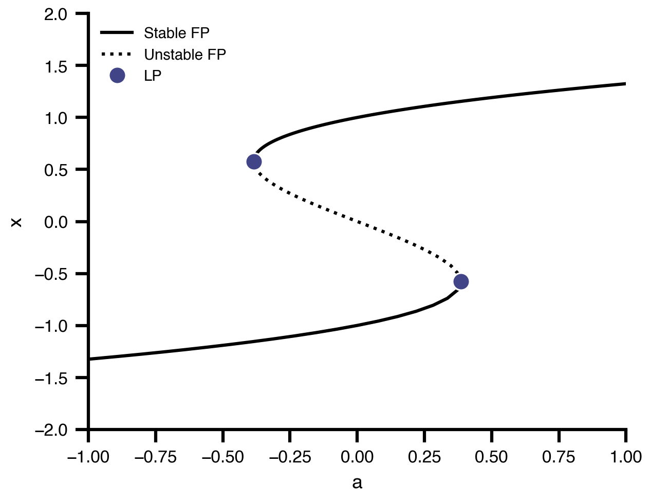

Forward and backward sweep — visualising the hysteresis loop

Numerically integrate the system while slowly sweeping \(a\) first up (\(-1 \to 1\)) then back down (\(1 \to -1\)). Trajectories track the upper branch on the way up and the lower branch on the way down — the system remembers its history.

def sweep(dyn, a_start, a_end, n_steps=4000, x0=1.0):
    rhs = lambda x, a: a + x - x**3
    a_traj = np.linspace(a_start, a_end, n_steps)
    x = np.empty(n_steps); x[0] = x0
    dt = 0.05
    for k in range(1, n_steps):
        x[k] = x[k-1] + dt * rhs(x[k-1], a_traj[k-1])
    return a_traj, x

a_up,   x_up   = sweep(dyn, -1.0, +1.0, x0=-1.0)
a_down, x_down = sweep(dyn, +1.0, -1.0, x0=+1.0)

fig, ax = plt.subplots(figsize=(6, 4))
ax.plot(a_up, x_up, color="C0", lw=2, label=r"sweep $a:-1\to 1$ (start low)")
ax.plot(a_down, x_down, color="C3", lw=2, label=r"sweep $a:+1\to -1$ (start high)")
af = 2.0/(3.0*np.sqrt(3.0))
ax.axvline(+af, color="0.5", ls="--", lw=0.8)
ax.axvline(-af, color="0.5", ls="--", lw=0.8)
ax.set_xlabel("$a$"); ax.set_ylabel("$x$")
ax.set_xlim(-1, 1); ax.set_ylim(-2, 2)
ax.legend(loc="upper left", fontsize=9, handlelength=1.4)
plt.tight_layout(); plt.show()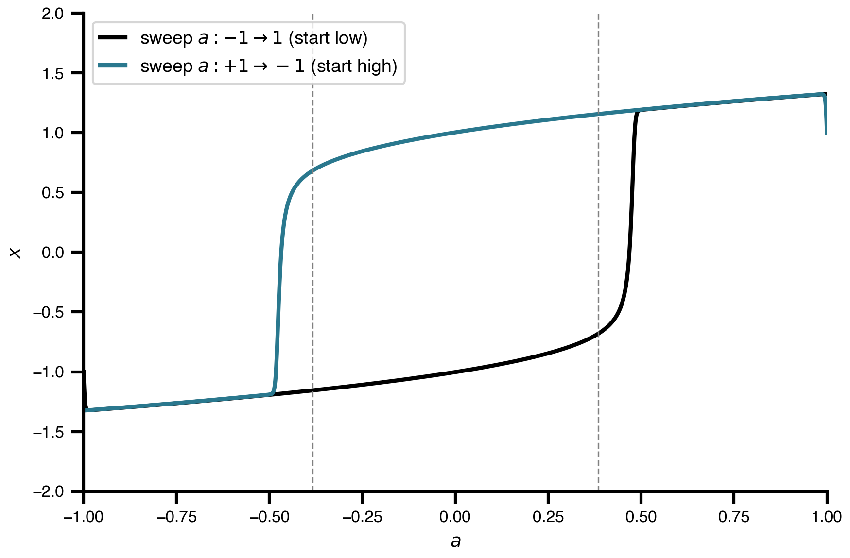

The system jumps discontinuously to the opposite branch precisely when each saddle-node is crossed. The enclosed area of the loop is the hysteresis area — a quantitative measure of memory.