Heterogeneous Kuramoto Oscillators

Phase oscillators with heterogeneous frequencies on a ring network

Replicates the NetworkDynamics.jl Heterogeneous System tutorial — Kuramoto phase oscillators on an 8-node ring with heterogeneous natural frequencies.

YAML Specification

# =============================================================================
# Heterogeneous Kuramoto Oscillators
# =============================================================================
# Source: https://juliadynamics.github.io/NetworkDynamics.jl/stable/generated/heterogeneous_system/
#
# Kuramoto phase oscillators on a ring (Watts-Strogatz k=2, p=0) with
# heterogeneous natural frequencies and sinusoidal coupling K sin(theta_j - theta_i).
# =============================================================================

id: 101
label: "Heterogeneous Kuramoto Oscillators"
description: >
    Kuramoto model on an 8-node ring network.  Each oscillator has a natural
    frequency omega_0 and is coupled to its nearest neighbours via
    K sin(theta_src - theta_dst).  Demonstrates heterogeneous per-node parameters.
    Recreates the NetworkDynamics.jl Heterogeneous System tutorial.
references:
    - "https://juliadynamics.github.io/NetworkDynamics.jl/stable/generated/heterogeneous_system/"
    - "Kuramoto, Y. (1975). Self-entrainment of a population of coupled non-linear oscillators."

# -- Local Dynamics ------------------------------------------------------------
dynamics:
    name: Kuramoto
    label: "Kuramoto phase oscillator"
    description: >
        Single-variable phase oscillator: d(theta)/dt = omega_0 + sum(edges).
        The natural frequency omega_0 is a per-node parameter (heterogeneous).
    system_type: continuous
    autonomous: true
    parameters:
        omega0:
            label: "Natural frequency"
            symbol: "omega_0"
            value: 0.0
            unit: "rad/s"
            description: "Intrinsic angular frequency of the oscillator (heterogeneous per node)"
            distribution:
                name: Uniform
                domain: { lo: 0.2, hi: 1.0 }
    coupling_terms:
        c_coupling:
            description: "Aggregated sinusoidal coupling from incident edges"
    state_variables:
        theta:
            label: "Phase angle"
            symbol: "theta"
            equation:
                rhs: "omega0 + c_coupling"
                description: "d(theta)/dt = omega_0 + sum K sin(theta_j - theta_i)"
            initial_value: 0.0
            distribution:
                domain: { lo: 0, hi: 6.283185 }
            unit: "rad"
            variable_of_interest: true

# -- Network -------------------------------------------------------------------
network:
    label: "8-node ring (Watts-Strogatz k=2, p=0)"
    description: >
        Regular ring lattice: each node is connected to its 2 nearest
        neighbours on each side.  Equivalent to watts_strogatz(8, 2, 0)
        in Graphs.jl.
    number_of_nodes: 8
    graph_generator:
        name: watts_strogatz
        type: WattsStrogatz
        parameters:
            k: { name: k, value: 2 }
            p: { name: p, value: 0 }

    coupling:
        KuramotoCoupling:
            name: KuramotoCoupling
            label: "Kuramoto sinusoidal coupling"
            description: >
                Antisymmetric coupling: K sin(theta_src - theta_dst).
                The AntiSymmetric wrapper ensures g_src = -g_dst.
            delayed: false
            parameters:
                K:
                    label: "Coupling strength"
                    value: 3.0
                    unit: "1"
                    description: "Global coupling strength between oscillators"
            pre_expression:
                rhs: "K * sin(x_j - x_i)"
                description: "Kuramoto coupling: K sin(theta_j - theta_i)"


# -- Integration ---------------------------------------------------------------
integration:
    description: "Explicit Runge-Kutta (Tsit5) with dt=0.05 over t in [0, 10]"
    method: Tsit5
    step_size: 0.05
    duration: 10.0
    time_scale: "s"

Model Report

Heterogeneous Kuramoto Oscillators

Kuramoto model on an 8-node ring network. Each oscillator has a natural frequency omega_0 and is coupled to its nearest neighbours via K sin(theta_src - theta_dst). Demonstrates heterogeneous per-node parameters. Recreates the NetworkDynamics.jl Heterogeneous System tutorial.

1. Brain Network: 8-node ring (Watts-Strogatz k=2, p=0)

Regular ring lattice: each node is connected to its 2 nearest neighbours on each side. Equivalent to watts_strogatz(8, 2, 0) in Graphs.jl.

Regions: 8

Coupling: Kuramoto sinusoidal coupling

Antisymmetric coupling: K sin(theta_src - theta_dst). The AntiSymmetric wrapper ensures g_src = -g_dst.

Pre-synaptic: \(c_{\text{pre}} = - K \cdot \sin{\left(x_{i} - x_{j} \right)}\)

Parameter	Value	Description
\(K\)	3.0	Global coupling strength between oscillators

2. Local Dynamics: Kuramoto phase oscillator

Single-variable phase oscillator: d(theta)/dt = omega_0 + sum(edges). The model comprises 1 state variables.

2.1 State Equations

\[\dot{\theta} = c_{coupling} + \omega_{0}\]

2.2 Parameters

Parameter	Value	Unit	Description
\(\omega_{0}\)	0.0	rad_per_s	Intrinsic angular frequency of the oscillator (heterogeneous per node)

3. Numerical Integration

Method: Tsit5
Time step: \(\Delta t = 0.05\) ms
Duration: 10.0 ms

References

Kuramoto, Y. (1975). Self-entrainment of a population of coupled non-linear oscillators. Lecture Notes in Physics, 420-422.

Cabral, J., Hugues, E., Sporns, O., & Deco, G. (2011). Role of local network oscillations in resting-state functional connectivity. NeuroImage, 57(1), 130-139.

Strogatz, S. (2000). From kuramoto to crawford: exploring the onset of synchronization in populations of coupled oscillators. Physica D: Nonlinear Phenomena, 143(1–4), 1-20. - https://juliadynamics.github.io/NetworkDynamics.jl/stable/generated/heterogeneous_system/ - Kuramoto, Y. (1975). Self-entrainment of a population of coupled non-linear oscillators.

Generated Julia Code

# exp is already loaded in the 'Model Report' section above
Code(exp.render_code("networkdynamics"), language='julia')

using Graphs
using NetworkDynamics

using OrdinaryDiffEqTsit5







function Kuramoto_f!(dx, x, esum, (omega0,), t)
    theta = x[1]

    c_coupling = esum[1]
    dx[1] = c_coupling + omega0
    nothing
end

vertex_Kuramoto = VertexModel(;
    f = Kuramoto_f!,
    g = StateMask(1:1),
    sym = [:theta],
    psym = [:omega0 => 0.0],
    name = :Kuramoto,
)








function KuramotoCoupling_edge_g!(e_dst, v_src, v_dst, (K,), t)
    e_dst[1] = -K .* sin(v_dst[1] - v_src[1])
    nothing
end

edge_KuramotoCoupling = EdgeModel(;
    g = AntiSymmetric(KuramotoCoupling_edge_g!),
    outsym = [:coupling],
    psym = [:K => 3.0],
    name = :KuramotoCoupling,
)




g = watts_strogatz(8, 2, 0)


nw = Network(g, vertex_Kuramoto, edge_KuramotoCoupling)




s = NWState(nw)
using Random
rng = MersenneTwister(42)

for node in 1:nv(g)
    s.v[node, :theta] = 0 .+ (6.283185 - 0) .* rand(rng)
end
for node in 1:nv(g)
    s.p.v[node, :omega0] = 0.2 .+ (1.0 - 0.2) .* rand(rng)
end



tspan = (0.0, 10.0)
prob = ODEProblem(nw, uflat(s), tspan, pflat(s))
sol = solve(prob, Tsit5(); saveat=0.05)

adj_matrix = Float64.(adjacency_matrix(g))

using Random: MersenneTwister
function spring_layout(g; seed=42, iterations=50, k=1.0)
    rng = MersenneTwister(seed)
    n = nv(g)
    pos = randn(rng, n, 2)
    for _ in 1:iterations
        disp = zeros(n, 2)
        for i in 1:n, j in (i+1):n
            d = pos[i, :] - pos[j, :]
            dist = max(norm(d), 0.01)
            rep = k^2 / dist
            disp[i, :] .+= d / dist * rep
            disp[j, :] .-= d / dist * rep
        end
        for e in edges(g)
            i, j = src(e), dst(e)
            d = pos[j, :] - pos[i, :]
            dist = max(norm(d), 0.01)
            att = dist^2 / k
            disp[i, :] .+= d / dist * att
            disp[j, :] .-= d / dist * att
        end
        for i in 1:n
            dl = max(norm(disp[i, :]), 0.01)
            pos[i, :] .+= disp[i, :] / dl * min(dl, 0.1)
        end
    end
    return pos
end
using LinearAlgebra: norm
node_positions = spring_layout(g)

using Plots
plot(sol; ylabel="state", xlabel="time", title="Kuramoto on 8-node network")

Run & Plot

ts = exp.run(format="networkdynamics")
ts.plot()

Detected IPython. Loading juliacall extension. See https://juliapy.github.io/PythonCall.jl/stable/compat/#IPython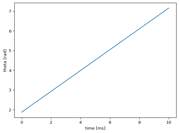

Results

Shape: (201, 1, 8)
Time range: 0.0 – 10.0
Final theta range: [6.293, 12.570]

Animate

ani = ts.animate("theta", format="dots")
ani.save("kuramoto.gif", writer="pillow", fps=20)