Parameter Continuation and Bifurcation Detection with TVBO

In this tutorial, you will learn how to perform a 1D numerical parameter continuation with automatic fold bifurcation detection using TVBO for model specification and PyRates/PyCoBi for the continuation analysis.

import os

import matplotlib.pyplot as plt
from pycobi import ODESystem
from pyrates import CircuitTemplate
from IPython.display import Markdown
from tvbo import Dynamics

qif_model = Dynamics.from_string(
    """
name: QIF
description: Quadratic Integrate-and-Fire (QIF) population mean-field model.
parameters:
    tau:
        value: 1.0
        description: Population time constant
    eta:
        value: -5.0
        description: mean of a Lorentzian distribution over the neural excitability
    Delta:
        value: 1.0
        description: half-width of a Lorentzian distribution over the neural excitability
    J:
        value: 15.0
        description: strength of the recurrent coupling inside the population
    
state_variables:
    r:
        description:  Average firing rate
        equation:
            rhs: Delta/(tau*pi) + 2*r*v
        initial_value: 0.1
    v:
        description: Average membrane potential
        equation:
            rhs: v**2 + eta + J*r*tau - (pi*r*tau)**2
        initial_value: -2.0

references:
    - Montbriot2015
"""
)

Markdown(qif_model.generate_report())

QIF

Quadratic Integrate-and-Fire (QIF) population mean-field model.

State Equations

\[ \frac{d}{d t} r = 2*r*v + \frac{\Delta}{\pi*\tau} \] \[ \frac{d}{d t} v = \eta + v^{2} + J*r*\tau - \pi^{2}*r^{2}*\tau^{2} \]

Parameters

Parameter Value Unit Description
\(\tau\) 1.0 N/A Population time constant
\(\eta\) -5.0 N/A mean of a Lorentzian distribution over the neural excitability
\(\Delta\) 1.0 N/A half-width of a Lorentzian distribution over the neural excitability
\(J\) 15.0 N/A strength of the recurrent coupling inside the population
# Export to PyRates YAML format
os.makedirs('_qif_model', exist_ok=True)
with open('_qif_model/__init__.py', 'w') as f:
    f.write('')

qif_model.to_yaml(format="pyrates", filepath='_qif_model/qif.yaml')
print("Model exported to PyRates format")
Model exported to PyRates format

Step 2: Generate Fortran Routines for AUTO-07p

Next, we translate the model into a Fortran file containing all subroutines required by AUTO-07p. This requires using the Fortran backend of PyRates with vectorize=False:

# Load the TVBO-exported model into PyRates
qif = CircuitTemplate.from_yaml("_qif_model.qif.QIF_circuit")

# Generate Fortran file with AUTO-07p subroutines
# Setting auto=True creates two files: .f90 (Fortran code) and c.ivp (AUTO constants)
qif.get_run_func(
    func_name='qif_rhs',
    file_name='qif',
    step_size=1e-4,
    auto=True,
    backend='fortran',
    solver='scipy',
    vectorize=False,
    float_precision='float64'
)
Compilation Progress
--------------------
    (1) Translating the circuit template into a networkx graph representation...
        ...finished.
    (2) Preprocessing edge transmission operations...
        ...finished.
    (3) Parsing the model equations into a compute graph...
        ...finished.
    Model compilation was finished.
(<fortran function qif_rhs>,
 (array(0.),
  array([ 0.1, -2. ]),
  array([0., 0.]),
  array(1.),
  array(1.),
  array(15.),
  array(-5.)),
 ('t',
  'y',
  'dy',
  'p/QIF_op/tau',
  'p/QIF_op/Delta',
  'p/QIF_op/J',
  'p/QIF_op/eta'),
 {'p/QIF_op/r': 0, 'p/QIF_op/v': 1})

Calling get_run_func with auto=True creates two files. The first is a .f90 file containing the Fortran subroutines:

f = open('qif.f90', 'r')
print(f.read())
f.close()
module qif

double precision :: PI = 4.0*atan(1.0)
complex :: I = (0.0, 1.0)

contains


subroutine qif_rhs(t,y,dy,tau,Delta,J,eta)

implicit none

double precision, intent(in) :: t
double precision, intent(in) :: y(2)
double precision :: r
double precision :: v
double precision, intent(inout) :: dy(2)
double precision, intent(in) :: tau
double precision, intent(in) :: Delta
double precision, intent(in) :: J
double precision, intent(in) :: eta


r = y(1)
v = y(2)

dy(1) = Delta/(pi*tau) + 2*r*v
dy(2) = J*r*tau + eta - pi**2*r**2*tau**2 + v**2

end subroutine


end module


subroutine func(ndim,y,icp,args,ijac,dy,dfdu,dfdp)

use qif
implicit none
integer, intent(in) :: ndim, icp(*), ijac
double precision, intent(in) :: y(ndim), args(*)
double precision, intent(out) :: dy(ndim)
double precision, intent(inout) :: dfdu(ndim,ndim), dfdp(ndim,*)

call qif_rhs(args(14), y, dy, args(1), args(2), args(3), args(4))

end subroutine func


subroutine stpnt(ndim, y, args, t)

implicit None
integer, intent(in) :: ndim
double precision, intent(inout) :: y(ndim), args(*)
double precision, intent(in) :: t

args(1) = 1.0  ! tau
args(2) = 1.0  ! Delta
args(3) = 15.0  ! J
args(4) = -5.0  ! eta
y(1) = 0.1  ! r
y(2) = -2.0  ! v

end subroutine stpnt


subroutine bcnd
end subroutine bcnd


subroutine icnd
end subroutine icnd


subroutine fopt
end subroutine fopt


subroutine pvls
end subroutine pvls

The second file contains the AUTO-07p parameters that determine how it performs parameter continuations:

f = open('c.ivp', 'r')
print(f.read())
f.close()
NDIM = 2
NPAR = 4
IPS = -2
ILP = 0
ICP = [14]
NTST = 1
NCOL = 3
IAD = 0
ISP = 0
ISW = 1
IPLT = 0
NBC = 0
NINT = 0
NMX = 9000
NPR = 20
MXBF = 10
IID = 2
ITMX = 2
ITNW = 5
NWTN = 2
JAC = 0
EPSL = 1e-06
EPSU = 1e-06
EPSS = 0.0001
IRS = 0
DS = 0.0001
DSMIN = 1e-08
DSMAX = 0.01
IADS = 1
THL = {}
THU = {}
UZR = {}
STOP = {}

The default parameters allow solving the initial value problem (performing simulations). For detailed explanation of these parameters, see the AUTO-07p documentation.

Step 3: Generate a PyCoBi Instance

Now that the model equations are compiled, we generate an instance of pycobi.ODESystem, which provides an interface to AUTO-07p:

qif_auto = ODESystem(eq_file="qif", working_dir=None, init_cont=False)

-------------------------------------------------------------
Could not import plotting modules, plotting will be disabled.
This is probably because Tkinter is not enabled in your Python installation.
-------------------------------------------------------------

Now we can use all tools provided by AUTO-07p to investigate how the model reacts to changes in its parameterization.

Part 2: Performing Parameter Continuations

Step 1: Time Continuation

In parameter continuations, we must start from an equilibrium or periodic orbit. We run a time continuation to let the system converge to an equilibrium:

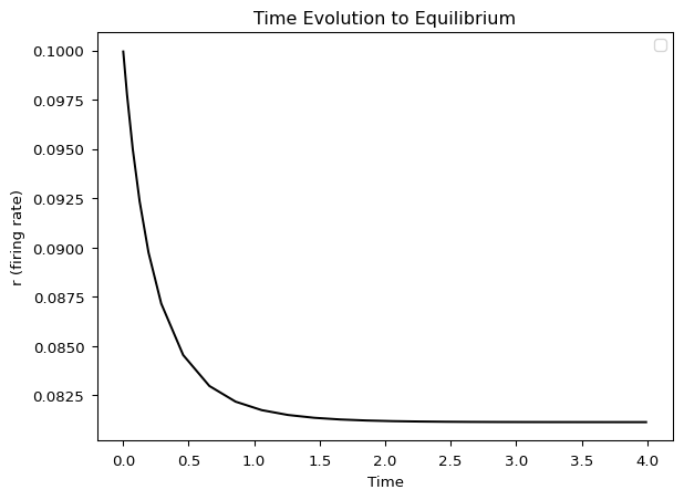
# Time continuation: integrate until system converges to equilibrium
t_sols, t_cont = qif_auto.run(
    c='ivp', name='time',
    DS=1e-4, DSMIN=1e-10, DSMAX=1e-2,
    EPSL=1e-08, EPSU=1e-08, EPSS=1e-06,
    NMX=1000,
    UZR={14: 4.0},   # Create marker when time (PAR 14) reaches 4.0
    STOP={'UZ1'}     # Stop at first user marker
)

# Plot time evolution
qif_auto.plot_continuation('PAR(14)', 'U(1)', cont='time')
plt.xlabel('Time')
plt.ylabel('r (firing rate)')
plt.title('Time Evolution to Equilibrium')
plt.show()
gfortran -g -fopenmp -O -c qif.f90 -o qif.o
gfortran -g -fopenmp -O qif.o -o qif.exe /Applications/auto-07p/lib/*.o
Starting qif ...

  BR    PT  TY  LAB    PAR(14)       L2-NORM         U(1)          U(2)     
   1     1  EP    1   0.00000E+00   2.00250E+00   1.00000E-01  -2.00000E+00
   1    20        2   2.97235E-02   1.99165E+00   9.77522E-02  -1.98925E+00
   1    40        3   7.34782E-02   1.97917E+00   9.49818E-02  -1.97689E+00
   1    60        4   1.25882E-01   1.96849E+00   9.23394E-02  -1.96633E+00
   1    80        5   1.93602E-01   1.95964E+00   8.97448E-02  -1.95759E+00
   1   100        6   2.90740E-01   1.95324E+00   8.71506E-02  -1.95129E+00
   1   120        7   4.58082E-01   1.95095E+00   8.45402E-02  -1.94912E+00
   1   140        8   6.58061E-01   1.95319E+00   8.29707E-02  -1.95143E+00
   1   160        9   8.58037E-01   1.95619E+00   8.21742E-02  -1.95446E+00
   1   180       10   1.05802E+00   1.95860E+00   8.17431E-02  -1.95690E+00
   1   200       11   1.25801E+00   1.96029E+00   8.14983E-02  -1.95860E+00
   1   220       12   1.45801E+00   1.96141E+00   8.13547E-02  -1.95972E+00
   1   240       13   1.65801E+00   1.96212E+00   8.12688E-02  -1.96043E+00
   1   260       14   1.85801E+00   1.96257E+00   8.12168E-02  -1.96088E+00
   1   280       15   2.05801E+00   1.96284E+00   8.11850E-02  -1.96116E+00
   1   300       16   2.25801E+00   1.96302E+00   8.11656E-02  -1.96134E+00
   1   320       17   2.45801E+00   1.96312E+00   8.11536E-02  -1.96145E+00
   1   340       18   2.65801E+00   1.96319E+00   8.11462E-02  -1.96151E+00
   1   360       19   2.85801E+00   1.96323E+00   8.11417E-02  -1.96155E+00
   1   380       20   3.05801E+00   1.96326E+00   8.11389E-02  -1.96158E+00
   1   400       21   3.25801E+00   1.96327E+00   8.11372E-02  -1.96159E+00
   1   420       22   3.45801E+00   1.96328E+00   8.11361E-02  -1.96160E+00
   1   440       23   3.65801E+00   1.96329E+00   8.11355E-02  -1.96161E+00
   1   460       24   3.85801E+00   1.96329E+00   8.11351E-02  -1.96161E+00
   1   475  UZ   25   4.00000E+00   1.96329E+00   8.11349E-02  -1.96162E+00

 Total Time    0.157E-01
qif ... done
/Users/leonmartin_bih/tools/tvbo/.venv/lib/python3.13/site-packages/pycobi/pycobi.py:677: UserWarning: No artists with labels found to put in legend.  Note that artists whose label start with an underscore are ignored when legend() is called with no argument.
  ax.legend()

Key parameters explained:

  • DS=1e-4: Initial step-size (in time units)
  • DSMIN=1e-10: Minimum step-size
  • DSMAX=1e-2: Maximum step-size
  • NMX=1000: Maximum number of continuation steps
  • UZR={14: 4.0}: Create user marker when parameter 14 (time) reaches 4.0
  • STOP={'UZ1'}: Stop at first user marker

The values for U(1) and U(2) converged to certain values, representing \(r\) and \(v\) at equilibrium.

Step 2: Continuation of \(\bar\eta\)

Now we perform the parameter continuation in \(\bar\eta\):

# Parameter continuation in eta (parameter 4)
eta_sols, eta_cont = qif_auto.run(
    origin=t_cont, starting_point='UZ1', name='eta',
    bidirectional=True,
    ICP=4,              # Continue parameter 4 (eta)
    RL0=-20.0,          # Lower bound for eta
    RL1=20.0,           # Upper bound for eta
    IPS=1,              # Equilibrium continuation
    ILP=1,              # Detect fold bifurcations
    ISP=2,              # Full automatic bifurcation detection
    ISW=1, NTST=400, NCOL=4, IAD=3, IPLT=0, NBC=0, NINT=0,
    NMX=2000, NPR=10, MXBF=5, IID=2, ITMX=40, ITNW=40, NWTN=12, JAC=0,
    EPSL=1e-06, EPSU=1e-06, EPSS=1e-04,
    DS=1e-4, DSMIN=1e-8, DSMAX=5e-2, IADS=1,
    THL={}, THU={}, UZR={}, STOP={}
)
Starting qif ...

  BR    PT  TY  LAB    PAR(4)        L2-NORM         U(1)          U(2)     
   1    10       26  -4.96775E+00   1.95372E+00   8.15337E-02  -1.95201E+00
   1    20       27  -4.53619E+00   1.81796E+00   8.76480E-02  -1.81584E+00
   1    30       28  -4.06624E+00   1.64837E+00   9.67195E-02  -1.64553E+00
   1    40       29  -3.61090E+00   1.44424E+00   1.10524E-01  -1.44000E+00
   1    50       30  -3.20876E+00   1.15754E+00   1.38489E-01  -1.14922E+00
   1    54  LP   31  -3.13613E+00   9.92398E-01   1.62570E-01  -9.78992E-01
   1    60       32  -3.30256E+00   7.78650E-01   2.12461E-01  -7.49103E-01
   1    70       33  -3.76060E+00   6.31484E-01   2.81574E-01  -5.65232E-01
   1    80       34  -4.24352E+00   5.74086E-01   3.49389E-01  -4.55524E-01
   1    90       35  -4.73111E+00   5.66407E-01   4.24761E-01  -3.74693E-01
   1   100       36  -5.21754E+00   6.02443E-01   5.18314E-01  -3.07063E-01
   1   110       37  -5.68459E+00   7.15455E-01   6.75553E-01  -2.35592E-01
   1   113  LP   38  -5.74353E+00   7.82981E-01   7.53992E-01  -2.11083E-01
   1   120       39  -5.45720E+00   9.41642E-01   9.25817E-01  -1.71908E-01
   1   130       40  -4.97011E+00   1.04741E+00   1.03609E+00  -1.53611E-01
   1   140       41  -4.47650E+00   1.12392E+00   1.11482E+00  -1.42763E-01
   1   150       42  -3.98076E+00   1.18709E+00   1.17940E+00  -1.34946E-01
   1   160       43  -3.48396E+00   1.24215E+00   1.23546E+00  -1.28823E-01
   1   170       44  -2.98651E+00   1.29161E+00   1.28566E+00  -1.23792E-01
   1   180       45  -2.48864E+00   1.33689E+00   1.33154E+00  -1.19527E-01
   1   190       46  -1.99046E+00   1.37890E+00   1.37403E+00  -1.15831E-01
   1   200       47  -1.49206E+00   1.41827E+00   1.41380E+00  -1.12573E-01
   1   210       48  -9.93474E-01   1.45544E+00   1.45130E+00  -1.09664E-01
   1   220       49  -4.94749E-01   1.49073E+00   1.48688E+00  -1.07039E-01
   1   230       50   4.09247E-03   1.52442E+00   1.52082E+00  -1.04651E-01
   1   240       51   5.03031E-01   1.55669E+00   1.55331E+00  -1.02461E-01
   1   250       52   1.00205E+00   1.58772E+00   1.58454E+00  -1.00443E-01
   1   260       53   1.50114E+00   1.61763E+00   1.61463E+00  -9.85707E-02
   1   270       54   2.00029E+00   1.64655E+00   1.64370E+00  -9.68274E-02
   1   280       55   2.49950E+00   1.67456E+00   1.67185E+00  -9.51971E-02
   1   290       56   2.99875E+00   1.70174E+00   1.69916E+00  -9.36670E-02
   1   300       57   3.49804E+00   1.72816E+00   1.72570E+00  -9.22264E-02
   1   310       58   3.99737E+00   1.75389E+00   1.75153E+00  -9.08661E-02
   1   320       59   4.49673E+00   1.77897E+00   1.77671E+00  -8.95783E-02
   1   330       60   4.99613E+00   1.80345E+00   1.80129E+00  -8.83563E-02
   1   340       61   5.49555E+00   1.82738E+00   1.82529E+00  -8.71941E-02
   1   350       62   5.99500E+00   1.85078E+00   1.84878E+00  -8.60866E-02
   1   360       63   6.49447E+00   1.87369E+00   1.87176E+00  -8.50294E-02
   1   370       64   6.99396E+00   1.89615E+00   1.89429E+00  -8.40184E-02
   1   380       65   7.49347E+00   1.91817E+00   1.91637E+00  -8.30501E-02
   1   390       66   7.99300E+00   1.93978E+00   1.93805E+00  -8.21214E-02
   1   400       67   8.49255E+00   1.96101E+00   1.95933E+00  -8.12294E-02
   1   410       68   8.99211E+00   1.98187E+00   1.98024E+00  -8.03716E-02
   1   420       69   9.49168E+00   2.00238E+00   2.00080E+00  -7.95456E-02
   1   430       70   9.99127E+00   2.02256E+00   2.02103E+00  -7.87496E-02
   1   440       71   1.04909E+01   2.04242E+00   2.04093E+00  -7.79814E-02
   1   450       72   1.09905E+01   2.06198E+00   2.06054E+00  -7.72395E-02
   1   460       73   1.14901E+01   2.08126E+00   2.07985E+00  -7.65223E-02
   1   470       74   1.19898E+01   2.10026E+00   2.09889E+00  -7.58283E-02
   1   480       75   1.24894E+01   2.11899E+00   2.11766E+00  -7.51562E-02
   1   490       76   1.29891E+01   2.13747E+00   2.13617E+00  -7.45049E-02
   1   500       77   1.34887E+01   2.15570E+00   2.15444E+00  -7.38731E-02
   1   510       78   1.39884E+01   2.17370E+00   2.17247E+00  -7.32599E-02
   1   520       79   1.44881E+01   2.19148E+00   2.19027E+00  -7.26644E-02
   1   530       80   1.49878E+01   2.20904E+00   2.20786E+00  -7.20856E-02
   1   540       81   1.54875E+01   2.22639E+00   2.22524E+00  -7.15227E-02
   1   550       82   1.59872E+01   2.24353E+00   2.24241E+00  -7.09749E-02
   1   560       83   1.64869E+01   2.26048E+00   2.25939E+00  -7.04416E-02
   1   570       84   1.69866E+01   2.27725E+00   2.27617E+00  -6.99221E-02
   1   580       85   1.74863E+01   2.29383E+00   2.29278E+00  -6.94158E-02
   1   590       86   1.79861E+01   2.31023E+00   2.30920E+00  -6.89220E-02
   1   600       87   1.84858E+01   2.32646E+00   2.32546E+00  -6.84403E-02
   1   610       88   1.89855E+01   2.34253E+00   2.34154E+00  -6.79701E-02
   1   620       89   1.94853E+01   2.35843E+00   2.35747E+00  -6.75110E-02
   1   630       90   1.99850E+01   2.37418E+00   2.37324E+00  -6.70624E-02
   1   631  EP   91   2.00350E+01   2.37575E+00   2.37480E+00  -6.70181E-02

 Total Time    0.188E-01
qif ... done
Starting qif ...

  BR    PT  TY  LAB    PAR(4)        L2-NORM         U(1)          U(2)     
   1    10       26  -5.03226E+00   1.97282E+00   8.07417E-02  -1.97116E+00
   1    20       27  -5.46785E+00   2.09536E+00   7.60058E-02  -2.09399E+00
   1    30       28  -5.95176E+00   2.22084E+00   7.17018E-02  -2.21968E+00
   1    40       29  -6.43776E+00   2.33809E+00   6.80993E-02  -2.33710E+00
   1    50       30  -6.92534E+00   2.44867E+00   6.50193E-02  -2.44781E+00
   1    60       31  -7.41415E+00   2.55368E+00   6.23424E-02  -2.55292E+00
   1    70       32  -7.90398E+00   2.65392E+00   5.99850E-02  -2.65325E+00
   1    80       33  -8.39463E+00   2.75005E+00   5.78864E-02  -2.74944E+00
   1    90       34  -8.88599E+00   2.84254E+00   5.60012E-02  -2.84199E+00
   1   100       35  -9.37794E+00   2.93182E+00   5.42947E-02  -2.93132E+00
   1   110       36  -9.87041E+00   3.01820E+00   5.27397E-02  -3.01774E+00
   1   120       37  -1.03633E+01   3.10197E+00   5.13147E-02  -3.10155E+00
   1   130       38  -1.08567E+01   3.18336E+00   5.00020E-02  -3.18297E+00
   1   140       39  -1.13503E+01   3.26258E+00   4.87875E-02  -3.26221E+00
   1   150       40  -1.18443E+01   3.33978E+00   4.76592E-02  -3.33944E+00
   1   160       41  -1.23386E+01   3.41513E+00   4.66072E-02  -3.41481E+00
   1   170       42  -1.28332E+01   3.48876E+00   4.56233E-02  -3.48846E+00
   1   180       43  -1.33279E+01   3.56078E+00   4.47002E-02  -3.56050E+00
   1   190       44  -1.38229E+01   3.63130E+00   4.38318E-02  -3.63104E+00
   1   200       45  -1.43181E+01   3.70041E+00   4.30129E-02  -3.70016E+00
   1   210       46  -1.48135E+01   3.76820E+00   4.22390E-02  -3.76796E+00
   1   220       47  -1.53091E+01   3.83474E+00   4.15059E-02  -3.83451E+00
   1   230       48  -1.58048E+01   3.90009E+00   4.08102E-02  -3.89988E+00
   1   240       49  -1.63006E+01   3.96433E+00   4.01488E-02  -3.96413E+00
   1   250       50  -1.67966E+01   4.02751E+00   3.95189E-02  -4.02731E+00
   1   260       51  -1.72927E+01   4.08967E+00   3.89180E-02  -4.08949E+00
   1   270       52  -1.77890E+01   4.15088E+00   3.83441E-02  -4.15070E+00
   1   280       53  -1.82853E+01   4.21117E+00   3.77951E-02  -4.21100E+00
   1   290       54  -1.87818E+01   4.27058E+00   3.72692E-02  -4.27042E+00
   1   300       55  -1.92784E+01   4.32915E+00   3.67649E-02  -4.32900E+00
   1   310       56  -1.97750E+01   4.38692E+00   3.62806E-02  -4.38677E+00
   1   315  EP   57  -2.00234E+01   4.41552E+00   3.60457E-02  -4.41537E+00

 Total Time    0.954E-02
qif ... done
Merge done

Key parameters explained:

  • origin=t_cont: Start from time continuation branch
  • starting_point='UZ1': Start from first user marker
  • bidirectional=True: Continue in both positive and negative directions
  • ICP=4: Parameter index for \(\bar\eta\) (4th parameter in Fortran file)
  • RL0=-20.0, RL1=20.0: Parameter bounds
  • IPS=1: Indicates equilibrium continuation of an ODE system
  • ILP=1: Enable fold bifurcation detection
  • ISP=2: Full automatic bifurcation detection

The output shows LP in column TY for some solutions, indicating limit point (fold) bifurcations.

Part 3: Bifurcation Diagram

We can visualize the full bifurcation diagram:

# Plot bifurcation diagram
fig, axes = plt.subplots(1, 2, layout="compressed", figsize=(10, 5))

# Firing rate vs eta
ax = axes[0]
qif_auto.plot_continuation("PAR(4)", "U(1)", cont="eta", ax=ax)
ax.set_xlabel("η (Background drive)")
ax.set_ylabel("Firing rate r")
ax.set_title("QIF Bifurcation Diagram: Firing Rate")

# Membrane potential vs eta
ax = axes[1]
qif_auto.plot_continuation("PAR(4)", "U(2)", cont="eta", ax=ax)
ax.set_xlabel("η (Background drive)")
ax.set_ylabel("Membrane potential v")
ax.set_title("QIF Bifurcation Diagram: Voltage")
plt.show()

Interpreting the Diagram

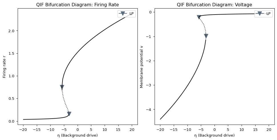
The curve represents the value of \(r\) (y-axis) at equilibrium solutions for each value of \(\bar\eta\) (x-axis):

  • Solid line: Stable equilibrium
  • Dotted line: Unstable equilibrium
  • Triangles (LP): Fold (limit point) bifurcations

At a fold bifurcation, the critical eigenvalue of the vector field crosses the imaginary axis (its real part changes sign), indicating a change of stability. A stable and unstable equilibrium approach and annihilate each other.

import shutil

# Clean up temporary files
qif.clear()
shutil.rmtree('_continuation', ignore_errors=True)

# Remove generated files
for f in ['qif.f90', 'c.ivp']:
    if os.path.exists(f):
        os.remove(f)

print("Cleaned up temporary files")
Cleaned up temporary files

References