from tvbo import Dynamics, Continuation, SimulationExperiment
import matplotlib.pyplot as plt
import numpy as np

PF_YAML = """
name: Pitchfork
description: Supercritical pitchfork $\\dot x = a x - x^3$.
parameters:
  a:
    name: a
    value: 1.0
state_variables:
  x:
    name: x
    domain: { lo: -2.0, hi: 2.0 }
    equation:
      lhs: Derivative(x, t)
      rhs: a*x - x**3
    initial_value: 0.01
"""

CONT_YAML = """
name: pf_in_a
dynamics: Pitchfork
free_parameters:
  - name: a
    domain: { lo: -1.0, hi: 2.0 }
max_steps: 400
ds: 0.005
bothside: true
"""

dyn = Dynamics.from_string(PF_YAML)
cont = Continuation.from_string(CONT_YAML)
exp = SimulationExperiment(dynamics=dyn, continuations=[cont])4. Pitchfork
The supercritical pitchfork bifurcation:
\[ \dot x = a\,x - x^3. \]
Equilibria: \(x = 0\) for all \(a\), plus \(x_{\pm} = \pm\sqrt{a}\) for \(a > 0\). The Jacobian at the trivial branch is \(f'(0) = a\), so \(x = 0\) is stable for \(a < 0\) and unstable for \(a > 0\). The two non-trivial branches inherit stability from the loss-of-stability of the trivial one.
This is the canonical symmetry-breaking bifurcation: the system has the symmetry \(x \mapsto -x\), and at the bifurcation point a pair of asymmetric solutions emerges from the symmetric one.
Phase line \(f(x)\) across the bifurcation
x = np.linspace(-2, 2, 400)
fig, axes = plt.subplots(1, 3, figsize=(12, 3.6), sharey=True)
for ax, a in zip(axes, [-0.5, 0.0, 1.0]):
    f = a*x - x**3
    ax.axhline(0, color="0.7", lw=0.8)
    ax.plot(x, f, lw=2, color="C0")
    eqs = [0.0]
    if a > 0:
        eqs += [+np.sqrt(a), -np.sqrt(a)]
    for r in eqs:
        slope = a - 3*r**2
        ax.plot(r, 0, "o", color="C2" if slope < 0 else "C3", ms=8, mec="k")
    ax.set_xlim(-2, 2); ax.set_ylim(-2.0, 2.0)
    ax.set_xlabel("$x$"); ax.set_title(f"$a = {a}$")
axes[0].set_ylabel(r"$\dot x = a x - x^3$")
plt.tight_layout(); plt.show()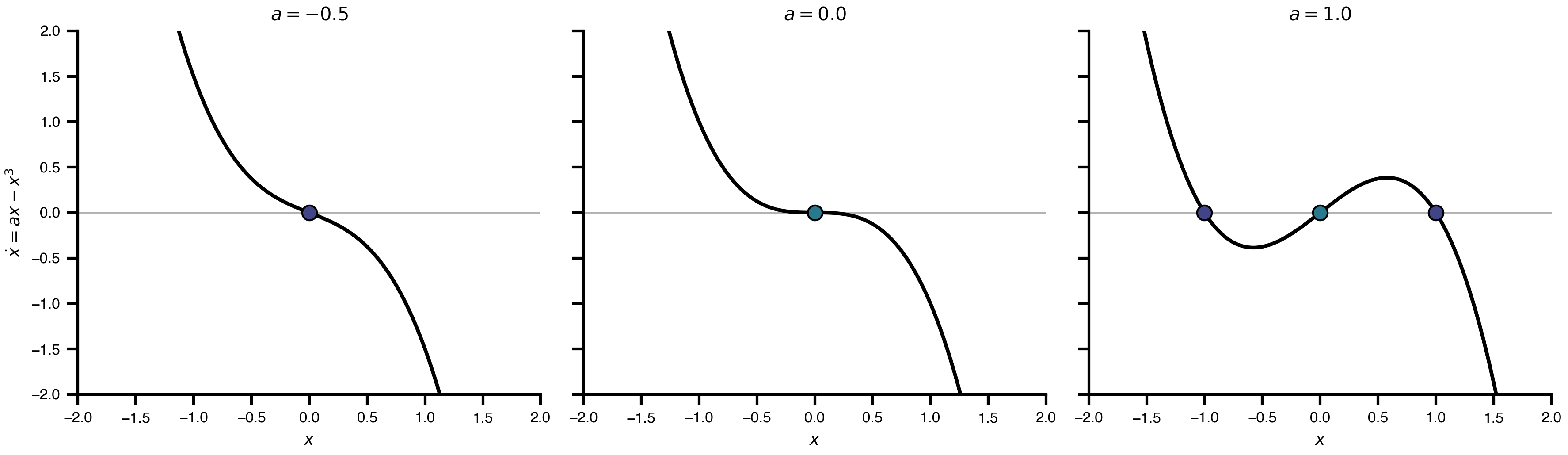
For \(a > 0\) the trivial equilibrium (red) is unstable and two new stable branches (green) flank it.
AUTO-07p (NumCont)
Mirrors the standalone PitchFork.py example: AUTO-07p time-integrates the YAML-defined system to a steady state, then continues in both directions of \(a\) via bothside: true.
result_auto = exp.run("auto-07p")
result_auto.continuations["pf_in_a"].plot(VOI="x")
plt.gca().set_xlim(-1, 2); plt.gca().set_ylim(-1.5, 1.5); plt.show()
/opt/homebrew/bin/gfortran -arch arm64 -O -fopenmp -O -c /var/folders/ym/9kw1g21j1nd7kwfn8c0z3st40000gn/T/tvbo_numcont_Pitchfork__vq26j6p/model.f90 -o /var/folders/ym/9kw1g21j1nd7kwfn8c0z3st40000gn/T/tvbo_numcont_Pitchfork__vq26j6p/model.o
/opt/homebrew/bin/gfortran -arch arm64 -O -fopenmp -O /var/folders/ym/9kw1g21j1nd7kwfn8c0z3st40000gn/T/tvbo_numcont_Pitchfork__vq26j6p/model.o -o /var/folders/ym/9kw1g21j1nd7kwfn8c0z3st40000gn/T/tvbo_numcont_Pitchfork__vq26j6p/model.exe /Applications/auto-07p/lib/*.o
Starting /var/folders/ym/9kw1g21j1nd7kwfn8c0z3st40000gn/T/tvbo_numcont_Pitchfork__vq26j6p/model ...ld: warning: duplicate -rpath '/Library/Developer/CommandLineTools/SDKs/MacOSX26.4.sdk/usr/lib' ignored
  BR    PT  TY  LAB       a          L2-NORM          x
   1     1  EP    1   1.00000E+00   1.00000E+00   1.00000E+00
   1    10        2   1.20109E+00   1.09594E+00   1.09594E+00
   1    20        3   1.55022E+00   1.24508E+00   1.24508E+00
   1    30  EP    4   2.04811E+00   1.43112E+00   1.43112E+00

 Total Time    0.991E-03
/var/folders/ym/9kw1g21j1nd7kwfn8c0z3st40000gn/T/tvbo_numcont_Pitchfork__vq26j6p/model ... done
Starting /var/folders/ym/9kw1g21j1nd7kwfn8c0z3st40000gn/T/tvbo_numcont_Pitchfork__vq26j6p/model ...

  BR    PT  TY  LAB       a          L2-NORM          x
   1     1  EP    1   1.00000E+00   1.00000E+00   1.00000E+00
   1    10        2   8.02934E-01   8.96066E-01   8.96066E-01
   1    20        3   4.81697E-01   6.94044E-01   6.94044E-01
   1    30        4   1.97049E-01   4.43902E-01   4.43902E-01
   1    40        5   1.34522E-02   1.15984E-01   1.15984E-01
   1    44  BP    6   5.51118E-09   1.11387E-09   1.11387E-09
   1    50        7   4.87844E-02   2.20872E-01  -2.20872E-01
   1    60        8   2.74087E-01   5.23533E-01  -5.23533E-01
   1    70        9   5.72943E-01   7.56930E-01  -7.56930E-01
   1    80       10   9.00364E-01   9.48875E-01  -9.48875E-01
   1    90       11   1.24198E+00   1.11444E+00  -1.11444E+00
   1   100       12   1.59191E+00   1.26171E+00  -1.26171E+00
   1   108  EP   13   2.00091E+00   1.41453E+00  -1.41453E+00

  BR    PT  TY  LAB       a          L2-NORM          x
   2    10       14  -4.60000E-01   5.96950E-68   5.96950E-68
   2    16  EP   15  -1.06000E+00   1.23082-109  -1.23082-109

  BR    PT  TY  LAB       a          L2-NORM          x
   2    10       16   4.60000E-01   5.73768E-68   5.73768E-68
   2    20       17   1.46000E+00   7.05377-138   7.05377-138
   2    26  EP   18   2.06000E+00   0.00000E+00   1.23508-180

 Total Time    0.175E-02
/var/folders/ym/9kw1g21j1nd7kwfn8c0z3st40000gn/T/tvbo_numcont_Pitchfork__vq26j6p/model ... done
Merge done
Saving to pf_in_a, pf_in_a, and pf_in_a ... done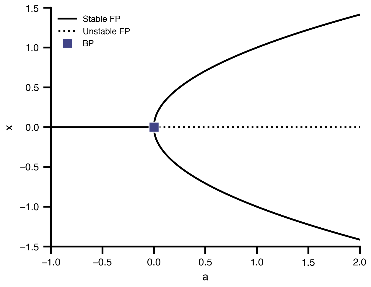
3D bifurcation surface \((a, x, t)\)
A pedagogical view: integrate the system from a small positive perturbation across a finite time horizon for many values of \(a\), and stack the trajectories along the \(a\)-axis. The convergence to \(x \to +\sqrt a\) for \(a > 0\) and to \(x \to 0\) for \(a < 0\) is visible as a 3-D surface.
from mpl_toolkits.mplot3d import Axes3D  # noqa: F401
a_grid = np.linspace(-1, 2, 60)
t = np.linspace(0, 8, 200)
X = np.empty((len(a_grid), len(t)))
for i, a in enumerate(a_grid):
    # closed-form for $\dot x = a x - x^3$ via separation
    x0 = 0.05
    if abs(a) < 1e-6:
        X[i] = x0 / np.sqrt(1 + 2 * x0**2 * t)
    else:
        c = (1.0 / x0**2 - a) if x0 != 0 else 1.0
        X[i] = a / np.sqrt(a + c * np.exp(-2*a*t)) * np.sign(x0)

fig = plt.figure(figsize=(7, 5))
ax = fig.add_subplot(111, projection="3d")
A_mesh, T_mesh = np.meshgrid(a_grid, t, indexing="ij")
ax.plot_surface(A_mesh, T_mesh, X, cmap="viridis", alpha=0.85,
                rcount=40, ccount=40)
ax.set_xlabel("$a$"); ax.set_ylabel("$t$"); ax.set_zlabel("$x(t)$")
ax.set_xlim(-1, 2); ax.set_zlim(-1.5, 1.5)
plt.tight_layout(); plt.show()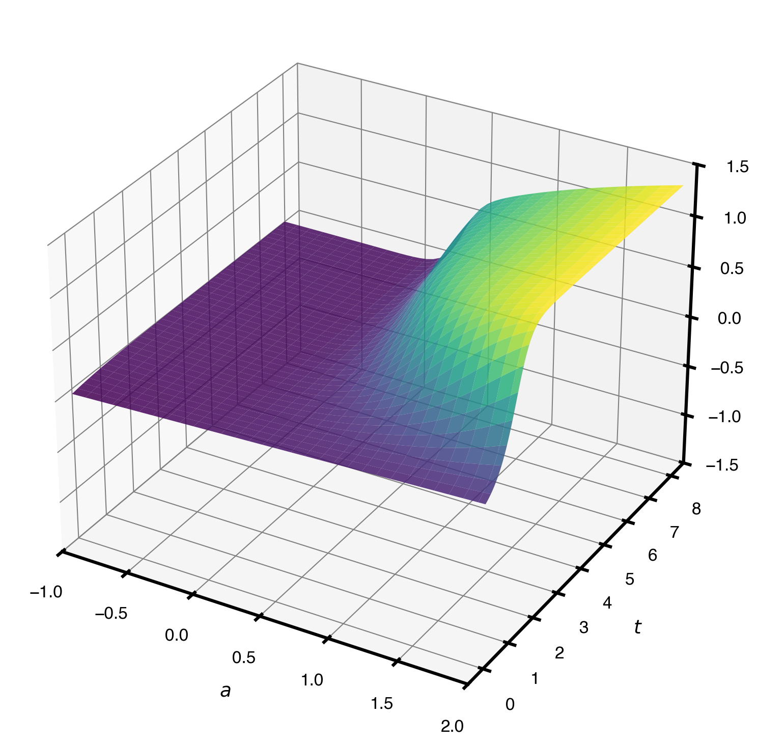
Note that detecting all three branches with continuation typically requires starting from a non-zero initial guess so that branch-switching at the pitchfork point is triggered. All backends label the bifurcation point at \(a = 0\).