PyRates Interoperability

This guide demonstrates full round-trip interoperability between TVBO and PyRates, a Python toolbox for dynamical systems modeling.

Overview

PyRates is a powerful framework for:

• Numerical simulation of dynamical systems
• Bifurcation analysis
• Parameter fitting
• Code generation (NumPy, TensorFlow, Julia, Fortran)

TVBO provides seamless bidirectional integration:

Direction	Method	Use Case
TVBO → PyRates	model.to_yaml(format="pyrates")	Use PyRates analysis tools
PyRates → TVBO	Dynamics.from_pyrates()	Use TVBO simulation/export

Feature Mapping

Feature	TVBO	PyRates
Differential equations	equation.rhs attribute	var' = rhs syntax
Initial values	initial_value attribute	variable(value)
Parameters	Parameter objects	Numeric values
Outputs	output	output marker
Inputs	coupling_terms	input(value) marker
Single node	Dynamics	NodeTemplate
Network	Network	CircuitTemplate

Round-Trip 1: TVBO → PyRates → TVBO

Step 1: Define Model in TVBO

from tvbo import Dynamics
from IPython.display import Markdown, display

# Create a Van der Pol oscillator model in TVBO
vdp = Dynamics("Dynamics")
vdp.name = "VanDerPol"
vdp.description = "Van der Pol oscillator - a classical nonlinear oscillator"

# Add parameters
vdp.add_parameter("mu", value=5.0, description="Damping constant")

# Add state variables with their differential equations
vdp.add_state_variable("x", equation="z", initial_value=0.0, description="Position")
vdp.add_state_variable("z", equation="mu*(1 - x**2)*z - x", initial_value=1.0, description="Velocity")

# Display model summary using generate_report
display(Markdown(vdp.generate_report(format="markdown")))

VanDerPol

Van der Pol oscillator - a classical nonlinear oscillator

State Equations

\[ \frac{d}{d t} x = z \] \[ \frac{d}{d t} z = - x + \mu*z*\left(1 - x^{2}\right) \]

Parameters

Parameter	Value	Unit	Description
\(\mu\)	5.0	N/A	Damping constant

Step 2: Export to PyRates and Simulate

import os
import shutil
import matplotlib.pyplot as plt
from pyrates import CircuitTemplate, clear

# Export TVBO model to PyRates format
os.makedirs('_pyrates_vdp', exist_ok=True)
with open('_pyrates_vdp/__init__.py', 'w') as f:
    f.write('')

pyrates_yaml = vdp.to_yaml(format="pyrates", filepath='_pyrates_vdp/vdp.yaml')

# Display exported code using render_code
print("=== Generated Python Code ===")
print(vdp.render_code(format="python"))

=== Generated Python Code ===
import numpy as np
import scipy


def VanDerPol(
    current_state,
    t,
    mu=5.0,
    local_coupling=0.0,
    stimulus=None,
    stimulus_scaling=1.0,
):
    e = np.e
    stim_t = stimulus_scaling * stimulus(t) if stimulus is not None else 0.0

    x = current_state[0]
    z = current_state[1]

    # Derived Variables

    # Time Derivatives
    next_state = np.array(
        [
            # x
            z,
            # z
            -x + mu * z * (1 - x**2),
        ]
    )

    return next_state

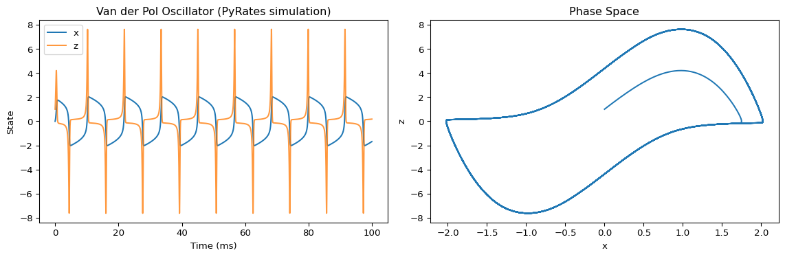
# Run in PyRates
T = 100.0
step_size = 1e-2

print("Running TVBO-exported model in PyRates...")
model = CircuitTemplate.from_yaml('_pyrates_vdp.vdp.VanDerPol_circuit')
results = model.run(
    step_size=step_size,
    simulation_time=T,
    outputs={'x': 'p/VanDerPol_op/x', 'z': 'p/VanDerPol_op/z'},
    solver='scipy',
    method='RK45'
)
clear(model)
shutil.rmtree('_pyrates_vdp')

# Plot results
fig, axes = plt.subplots(1, 2, figsize=(12, 4))

axes[0].plot(results['x'], label='x')
axes[0].plot(results['z'], label='z', alpha=0.8)
axes[0].set_xlabel('Time (ms)')
axes[0].set_ylabel('State')
axes[0].set_title('Van der Pol Oscillator (PyRates simulation)')
axes[0].legend()

axes[1].plot(results['x'], results['z'])
axes[1].set_xlabel('x')
axes[1].set_ylabel('z')
axes[1].set_title('Phase Space')

plt.tight_layout()
plt.show()

Running TVBO-exported model in PyRates...
Compilation Progress
--------------------
    (1) Translating the circuit template into a networkx graph representation...
        ...finished.
    (2) Preprocessing edge transmission operations...
        ...finished.
    (3) Parsing the model equations into a compute graph...
        ...finished.
    Model compilation was finished.
Simulation Progress
-------------------
     (1) Generating the network run function...
     (2) Processing output variables...
        ...finished.
     (3) Running the simulation...
        ...finished after 0.031563042000925634s.

Step 3: Load Back into TVBO

import tempfile
from IPython.display import Markdown, display

# Save to file and reload
with tempfile.TemporaryDirectory() as tmpdir:
    filepath = os.path.join(tmpdir, "vanderpol.yaml")
    vdp.to_yaml(format="pyrates", filepath=filepath)

    # Load back into TVBO
    loaded = Dynamics.from_pyrates(filepath)

    # Display loaded model using generate_report
    print("=== Loaded Model Report ===")
    display(Markdown(loaded.generate_report(format="markdown")))

=== Loaded Model Report ===

VanDerPol

Van der Pol oscillator - a classical nonlinear oscillator

State Equations

\[ \frac{d}{d t} x = z \] \[ \frac{d}{d t} z = - x + \mu*z*\left(1 - x^{2}\right) \]

Parameters

Parameter	Value	Unit	Description
\(\mu\)	5.0	N/A	None

Step 4: Run in TVBO

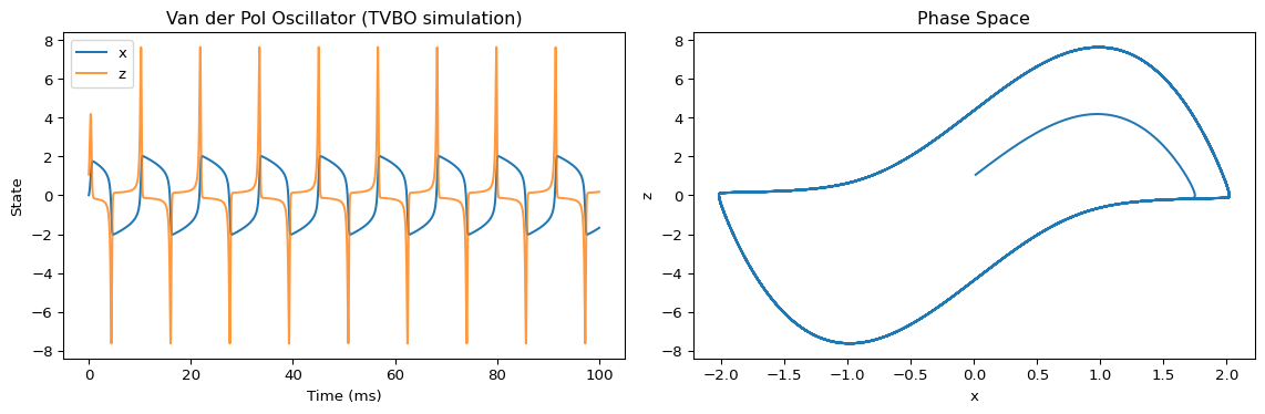
from tvbo import SimulationExperiment
from IPython.display import Markdown, display

# Run the loaded model in TVBO
exp = SimulationExperiment(
    local_dynamics=loaded,
)
exp.integration.duration=100

# Display experiment report
display(Markdown(exp.generate_report(format="markdown")))

result = exp.run()

# Plot TVBO simulation
fig, axes = plt.subplots(1, 2, figsize=(12, 4))

time = result.time
x = result.data[:, 0, 0, 0]
z = result.data[:, 1, 0, 0]

axes[0].plot(time, x, label="x")
axes[0].plot(time, z, label="z", alpha=0.8)
axes[0].set_xlabel("Time (ms)")
axes[0].set_ylabel("State")
axes[0].set_title("Van der Pol Oscillator (TVBO simulation)")
axes[0].legend()

axes[1].plot(x, z)
axes[1].set_xlabel("x")
axes[1].set_ylabel("z")
axes[1].set_title("Phase Space")

plt.tight_layout()
plt.show()

Simulation Experiment

---

Van der Pol oscillator - a classical nonlinear oscillator. The model comprises 2 state variables representing neural population activity.

\[\frac{dx}{dt} = z\]

\[\frac{dz}{dt} = - x + \mu \cdot z \cdot \left(1 - x^{2}\right)\]

Parameter	Value	Unit	Description
\(\mu\)	5.0	—

Pre-synaptic transformation: \[c_{\text{pre}} = x_{j}\]

Post-synaptic transformation: \[c_{\text{post}} = b + a \cdot gx\]

Parameter	Value	Description
\(b\)	0.0	Shifts the base of the connection strength while maintaining the absolute difference between different values.
\(a\)	0.00390625	Linear scaling factor of the coupled (delayed) input.

• Regions: 1

• Conduction velocity: 3.0 mm/ms

• Method: Heun

• Time step: \(\Delta t = 0.01220703125\) ms

• Duration: 100 ms

Round-Trip 2: PyRates → TVBO → PyRates

Step 1: Load PyRates Model into TVBO

from tvbo import Dynamics
from IPython.display import Markdown, display

# Load an existing PyRates model (Van der Pol oscillator from PyRates)
vdp_pyrates_path = "/Users/leonmartin_bih/work_data/toolboxes/PyRates/model_templates/oscillators/vanderpol.yaml"

# Load into TVBO (loads the first operator)
vdp_imported = Dynamics.from_pyrates(vdp_pyrates_path)

# Display using generate_report
display(Markdown(vdp_imported.generate_report(format="markdown")))

vdp

State Equations

\[ \frac{d}{d t} x = z \] \[ \frac{d}{d t} z = inp - x + \mu*z*\left(1 - x^{2}\right) \]

Parameters

Parameter	Value	Unit	Description
\(\mu\)	1.0	N/A	None
\(inp\)	0.0	N/A	None

Step 2: Modify in TVBO and Display Code

from IPython.display import Markdown, display

# Modify parameter in TVBO
vdp_imported.parameters['mu'].value = 2.5  # Change damping

# Display the generated Python code using render_code
print("=== Generated Python Code ===")
print(vdp_imported.render_code(format="python"))

=== Generated Python Code ===
import numpy as np
import scipy


def vdp(
    current_state,
    t,
    mu=2.5,
    inp=0.0,
    local_coupling=0.0,
    stimulus=None,
    stimulus_scaling=1.0,
):
    e = np.e
    stim_t = stimulus_scaling * stimulus(t) if stimulus is not None else 0.0

    x = current_state[0]
    z = current_state[1]

    # Derived Variables

    # Time Derivatives
    next_state = np.array(
        [
            # x
            z,
            # z
            inp - x + mu * z * (1 - x**2),
        ]
    )

    return next_state

Step 3: Run in TVBO

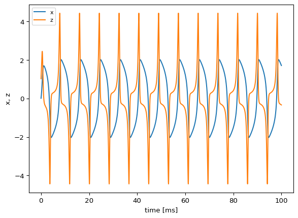
from IPython.display import Markdown, display

# Run the modified model in TVBO
exp = SimulationExperiment(
    local_dynamics=vdp_imported,
)
exp.integration.duration=100

# Display experiment configuration
Markdown(exp.generate_report(format="markdown"))

Simulation Experiment

---

The model comprises 2 state variables representing neural population activity.

\[\frac{dx}{dt} = z\]

\[\frac{dz}{dt} = inp - x + \mu \cdot z \cdot \left(1 - x^{2}\right)\]

Parameter	Value	Unit	Description
\(\mu\)	2.5	—
\(inp\)	0.0	—

Pre-synaptic transformation: \[c_{\text{pre}} = x_{j}\]

Post-synaptic transformation: \[c_{\text{post}} = b + a \cdot gx\]

Parameter	Value	Description
\(b\)	0.0	Shifts the base of the connection strength while maintaining the absolute difference between different values.
\(a\)	0.00390625	Linear scaling factor of the coupled (delayed) input.

• Regions: 1

• Conduction velocity: 3.0 mm/ms

• Method: Heun

• Time step: \(\Delta t = 0.01220703125\) ms

• Duration: 100 ms

result = exp.run()
result.plot()

Step 4: Export Back to PyRates

import tempfile

with tempfile.TemporaryDirectory() as tmpdir:
    # Export modified model back to PyRates
    filepath = os.path.join(tmpdir, "vdp_modified.yaml")
    vdp_imported.to_yaml(format="pyrates", filepath=filepath)

    # Display exported YAML
    print("=== Modified model exported to PyRates YAML ===")
    with open(filepath, 'r') as f:
        print(f.read())

=== Modified model exported to PyRates YAML ===

%YAML 1.2
---
# PyRates Experiment Template
# Generated from TVBO Dynamics
# This file is self-contained and ready for PyRates simulation.

# OPERATORS (Model Dynamics)


vdp_op:
  base: OperatorTemplate
  description: "TVBO model: vdp"
  equations:
    - "x' = z"
    - "z' = inp - x + mu*z*(1 - x**2)"
  variables:
    x: variable(0.0)
    z: variable(1.0)
    mu: 2.5
    inp: 0.0


# NODES (Network Topology)


vdp:
  base: NodeTemplate
  operators:
    - vdp_op

# CIRCUIT (Complete Network)

vdp_circuit:
  base: CircuitTemplate
  nodes:
    p: vdp

Loading Multi-Operator PyRates Files

PyRates files can contain multiple OperatorTemplates. Use SimulationExperiment.from_pyrates() to load all of them:

from tvbo import SimulationExperiment
from IPython.display import Markdown, display

# Load a multi-operator file (synaptic plasticity has 3 operators)
plasticity_path = "/Users/leonmartin_bih/work_data/toolboxes/PyRates/model_templates/neural_mass_models/synaptic_plasticity.yaml"

exp_multi = SimulationExperiment.from_pyrates(plasticity_path)

# Display each operator using generate_report
for name, dyn in exp_multi.dynamics.items():
    print(f"\n=== Operator: {name} ===")
    display(Markdown(dyn.generate_report(format="markdown")))

=== Operator: tsodyks ===

tsodyks

Derived Variables

\[ r_{eff} = r_{in}*u*x \]

State Equations

\[ \frac{d}{d t} x = \frac{1 - x}{\tau_{x}} - k*r_{in}*u*x \] \[ \frac{d}{d t} u = \frac{U_{0} - u}{\tau_{u}} + U_{0}*r_{in}*\left(1 - u\right) \]

Output Transforms

\[ r_{eff} = r_{in}*u*x \]

Parameters

Parameter	Value	Unit	Description
\(\tau_{x}\)	100.0	N/A	None
\(\tau_{u}\)	200.0	N/A	None
\(k\)	0.1	N/A	None
\(U_{0}\)	0.6	N/A	None
\(r_{in}\)	0.0	N/A	None

=== Operator: depression ===

depression

Derived Variables

\[ r_{eff} = r_{in}*x \]

State Equations

\[ \frac{d}{d t} x = \frac{1 - x}{\tau_{x}} - k*r_{in}*x \]

Output Transforms

\[ r_{eff} = r_{in}*x \]

Parameters

Parameter	Value	Unit	Description
\(\tau_{x}\)	100.0	N/A	None
\(k\)	1.0	N/A	None
\(r_{in}\)	0.0	N/A	None

=== Operator: facilitation ===

facilitation

Derived Variables

\[ r_{eff} = r_{in}*u \]

State Equations

\[ \frac{d}{d t} u = \frac{U_{0} - u}{\tau_{u}} - U_{0}*r_{in}*\left(1 - u\right) \]

Output Transforms

\[ r_{eff} = r_{in}*u \]

Parameters

Parameter	Value	Unit	Description
\(\tau_{u}\)	100.0	N/A	None
\(U_{0}\)	0.2	N/A	None
\(r_{in}\)	0.0	N/A	None

Run Tsodyks-Markram Synapse Model

from IPython.display import Markdown, display

# Run the Tsodyks-Markram model with constant presynaptic input
tsodyks = exp_multi.dynamics["tsodyks"]

# Set presynaptic firing rate (r_in is now a parameter since we loaded it)
if "r_in" in tsodyks.parameters:
    tsodyks.parameters["r_in"].value = 20.0  # 20 Hz input

# Display the rendered code
print("=== Generated Python Code for Tsodyks Model ===")
print(tsodyks.render_code(format="python"))

# Create experiment
synapse_exp = SimulationExperiment(
    local_dynamics=tsodyks
)

# Display experiment configuration
display(Markdown(synapse_exp.generate_report(format="markdown")))

result = synapse_exp.run()

# Plot synaptic dynamics
fig, axes = plt.subplots(1, 3, figsize=(14, 4))

time = result.time
x = result.data[:, 0, 0, 0]  # synaptic resources
u = result.data[:, 1, 0, 0]  # utilization factor

axes[0].plot(time, x)
axes[0].set_xlabel("Time (ms)")
axes[0].set_ylabel("x")
axes[0].set_title("Synaptic Resources (x)")

axes[1].plot(time, u)
axes[1].set_xlabel("Time (ms)")
axes[1].set_ylabel("u")
axes[1].set_title("Utilization Factor (u)")

# Effective rate = r_in * x * u
r_in = 20.0
r_eff = r_in * x * u
axes[2].plot(time, r_eff)
axes[2].set_xlabel("Time (ms)")
axes[2].set_ylabel("r_eff")
axes[2].set_title("Effective Rate (r_in × x × u)")
axes[2].axhline(r_in, color="gray", linestyle="--", label="Input rate")
axes[2].legend()

plt.tight_layout()
plt.show()

print(f"\nSteady-state depression: {x[-1]:.3f}")
print(f"Steady-state utilization: {u[-1]:.3f}")
print(f"Steady-state efficacy: {r_eff[-1]/r_in:.3f}")

=== Generated Python Code for Tsodyks Model ===
import numpy as np
import scipy


def tsodyks(
    current_state,
    t,
    tau_x=100.0,
    tau_u=200.0,
    k=0.1,
    U0=0.6,
    r_in=20.0,
    local_coupling=0.0,
    stimulus=None,
    stimulus_scaling=1.0,
):
    e = np.e
    stim_t = stimulus_scaling * stimulus(t) if stimulus is not None else 0.0

    x = current_state[0]
    u = current_state[1]

    # Derived Variables
    r_eff = r_in * u * x

    # Time Derivatives
    next_state = np.array(
        [
            # x
            (1 - x) / tau_x - k * r_in * u * x,
            # u
            (U0 - u) / tau_u + U0 * r_in * (1 - u),
        ]
    )

    return next_state

Simulation Experiment

---

The model comprises 2 state variables representing neural population activity.

\[r_{eff} = r_{in} \cdot u \cdot x\]

\[\frac{dx}{dt} = \frac{1 - x}{\tau_{x}} - k \cdot r_{in} \cdot u \cdot x\]

\[\frac{du}{dt} = \frac{U_{0} - u}{\tau_{u}} + U_{0} \cdot r_{in} \cdot \left(1 - u\right)\]

Parameter	Value	Unit	Description
\(\tau_{x}\)	100.0	—
\(\tau_{u}\)	200.0	—
\(k\)	0.1	—
\(U_{0}\)	0.6	—
\(r_{in}\)	20.0	—

Pre-synaptic transformation: \[c_{\text{pre}} = x_{j}\]

Post-synaptic transformation: \[c_{\text{post}} = b + a \cdot gx\]

Parameter	Value	Description
\(b\)	0.0	Shifts the base of the connection strength while maintaining the absolute difference between different values.
\(a\)	0.00390625	Linear scaling factor of the coupled (delayed) input.

• Regions: 1

• Conduction velocity: 3.0 mm/ms

• Method: Heun

• Time step: \(\Delta t = 0.01220703125\) ms

• Duration: 1000.0 ms

Steady-state depression: 0.100
Steady-state utilization: 0.100
Steady-state efficacy: 0.010

PyRates vs TVBO: Numerical Comparison

Let’s verify that both engines produce identical results:

import numpy as np
from IPython.display import Markdown, display

# Define identical model
mu_value = 3.0
T = 50.0
dt = 0.001  # Smaller step size for better accuracy

# Create TVBO model
vdp_compare = Dynamics("Dynamics")
vdp_compare.name = "VdP"
vdp_compare.add_parameter("mu", value=mu_value)
vdp_compare.add_state_variable("x", equation="z", initial_value=0.5)
vdp_compare.add_state_variable("z", equation="mu*(1 - x**2)*z - x", initial_value=0.5)

# Display model report
display(Markdown(vdp_compare.generate_report(format="markdown")))

# Run in TVBO (uses Heun by default)
exp_compare = SimulationExperiment(local_dynamics=vdp_compare)
exp_compare.integration.duration = T
exp_compare.integration.step_size = dt
tvbo_result = exp_compare.run()

# Run in PyRates with same solver (heun)
os.makedirs("_compare", exist_ok=True)
with open("_compare/__init__.py", "w") as f:
    f.write("")
vdp_compare.to_yaml(format="pyrates", filepath="_compare/model.yaml")

pyrates_model = CircuitTemplate.from_yaml("_compare.model.VdP_circuit")
pyrates_result = pyrates_model.run(
    step_size=dt,
    simulation_time=T + dt,
    outputs={"x": "p/VdP_op/x", "z": "p/VdP_op/z"},
    solver="heun",  # Use same solver as TVBO
)
clear(pyrates_model)
shutil.rmtree("_compare")

# Compare
tvbo_x = tvbo_result.data[:, 0, 0, 0]
tvbo_z = tvbo_result.data[:, 1, 0, 0]

fig, axes = plt.subplots(1, 2, layout='compressed')

axes[0].plot(tvbo_result.time, tvbo_x, label="TVBO")
axes[0].plot(pyrates_result["x"], "--", label="PyRates", alpha=0.8)
axes[0].set_xlabel("Time (ms)")
axes[0].set_ylabel("x")
axes[0].set_title("State Variable x")
axes[0].legend()

axes[1].plot(tvbo_result.time, tvbo_z, label="TVBO")
axes[1].plot(pyrates_result["z"], "--", label="PyRates", alpha=0.8)
axes[1].set_xlabel("Time (ms)")
axes[1].set_ylabel("z")
axes[1].set_title("State Variable z")
axes[1].legend()

for ax in fig.axes:
    ax.set_box_aspect(1)

VdP

State Equations

\[ \frac{d}{d t} x = z \] \[ \frac{d}{d t} z = - x + \mu*z*\left(1 - x^{2}\right) \]

Parameters

Parameter	Value	Unit	Description
\(\mu\)	3.0	N/A	None

Compilation Progress
--------------------
    (1) Translating the circuit template into a networkx graph representation...
        ...finished.
    (2) Preprocessing edge transmission operations...
        ...finished.
    (3) Parsing the model equations into a compute graph...
        ...finished.
    Model compilation was finished.
Simulation Progress
-------------------
     (1) Generating the network run function...
     (2) Processing output variables...
        ...finished.
     (3) Running the simulation...
        ...finished after 0.4788794580017566s.