Getting Started

From one equation to a whole-brain simulation

TVBO describes a simulation as data, not code. A model, a network, an integrator and whatever you want to measure are declared in one specification; TVBO generates the code and runs it on the backend you choose. The same file runs on JAX, TVB, PyRates, Julia or NeuroML, and it stays readable and version-controllable.

This page goes from a single equation to a whole-brain run in three steps. If you already know brain network modelling, skip to step 3 — the first two are the mechanics.

Imports and plot style

import warnings; warnings.filterwarnings("ignore")
import numpy as np
import matplotlib.pyplot as plt
import bsplot
from tvbo import SimulationExperiment, Dynamics

bsplot.style.use("tvbo")

Step 1: your first model

Any system of ODEs can be written directly. A damped oscillator,

\[ \dot{x} = v, \qquad \dot{v} = -k\,x - c\,v \]

becomes a specification by naming the state variables, their right-hand sides, and the parameters:

MINIMAL = """
label: "My first model"
dynamics:
  name: DampedOscillator
  state_variables:
    x:
      equation: {rhs: "v"}
      initial_value: 1.0
    v:
      equation: {rhs: "-k*x - c*v"}
      initial_value: 0.0
  parameters:
    k: {value: 1.0}      # stiffness
    c: {value: 0.1}      # damping
network:
  number_of_nodes: 1
integration:
  method: Heun
  step_size: 0.01
  duration: 40.0
"""

result = SimulationExperiment.from_string(MINIMAL).run()
x = result.integration.data.sel(variable="x").squeeze()
print(f"released at x = {float(x[0]):.2f}, settled to x = {float(x[-1]):.3f}")

INFO [tvbo.run] [+0s] STEP 1: Running simulation...
INFO [tvbo.run] [+0s]   Simulation period: 40.0 ms, dt: 0.01 ms
INFO [tvbo.run] [+0s]   Simulation complete.
INFO [tvbo.run] [+0s] Experiment complete.

released at x = 1.00, settled to x = -0.080

Code

fig, ax = plt.subplots(figsize=(8, 2.6))
ax.plot(x.time, x, lw=1.5)
ax.axhline(0, color="0.7", lw=0.6)
ax.set_xlabel("time")
ax.set_ylabel("$x$")
plt.tight_layout()
plt.show()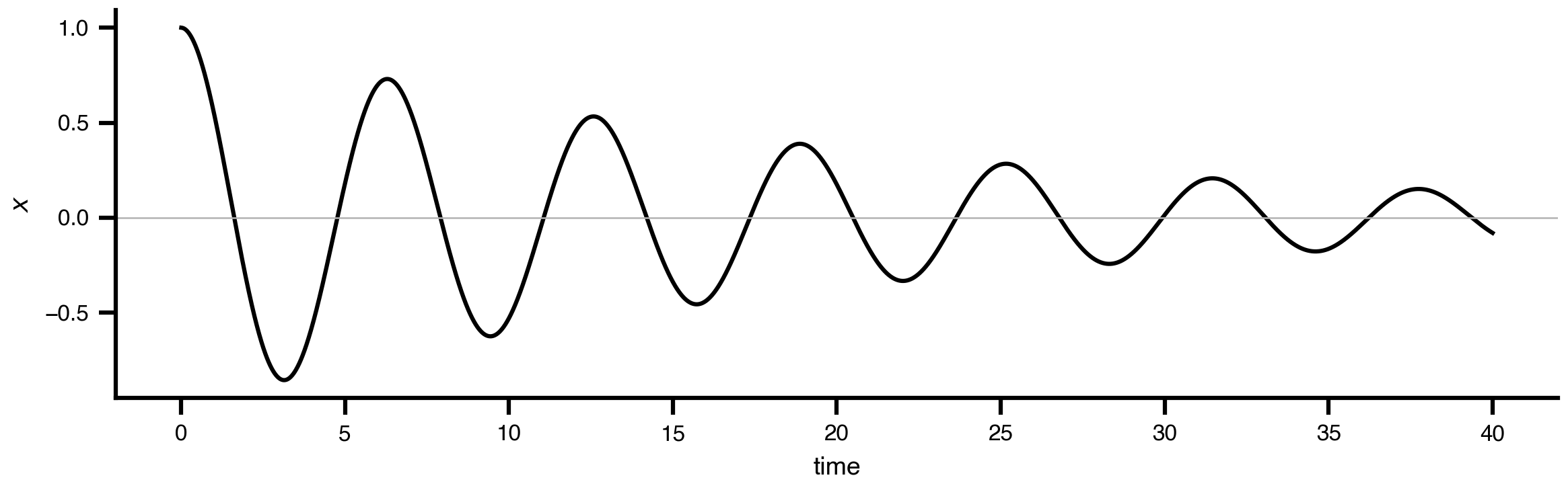

Figure 1: The damped oscillator, released from \(x=1\) and decaying toward rest.

That is the whole loop: declare → run → inspect. Everything after this is the same loop with richer ingredients.

Step 2: a model from the database

You rarely write neural mass models by hand — TVBO ships a curated library. Reference one by its ontology iri instead of spelling out the equations:

jr = Dynamics.from_db("JansenRit")
print("Jansen-Rit state variables:", list(jr.state_variables))
print("accepted coupling inputs :", list(jr.coupling_inputs))

Jansen-Rit state variables: ['y0', 'y1', 'y2', 'y3', 'y4', 'y5']
accepted coupling inputs : ['c_glob', 'local_coupling']

JR = """
label: "Jansen-Rit, one region"
dynamics:
  iri: tvbo:JansenRit
network:
  number_of_nodes: 1
integration:
  method: Heun
  step_size: 0.5
  duration: 2000.0
  transient_time: 500.0
"""
jr_res = SimulationExperiment.from_string(JR).run()
print("dims:", dict(zip(jr_res.integration.data.dims, jr_res.integration.data.shape)))

INFO [tvbo.run] [+0s] STEP 1: Running simulation...
INFO [tvbo.run] [+0s]   Simulation period: 2000.0 ms, dt: 0.5 ms
INFO [tvbo.run] [+0s]   Transient period: 500.0 ms (settled on (-500.0, 0], warm-started via update_history)
INFO [tvbo.run] [+0s]   Simulation complete.
INFO [tvbo.run] [+0s] Experiment complete.

dims: {'time': 4000, 'variable': 6}

Code

d = jr_res.integration.data
eeg = (d.sel(variable="y1") - d.sel(variable="y2")).squeeze()

fig, ax = plt.subplots(figsize=(8, 2.6))
ax.plot(eeg.time, eeg, lw=1.0)
ax.set_xlabel("time (ms)")
ax.set_ylabel("$y_1 - y_2$  (mV)")
plt.tight_layout()
plt.show()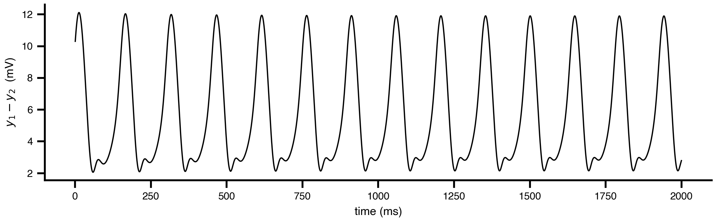

Figure 2: A single Jansen-Rit column. The pyramidal-cell potential is the difference \(y_1 - y_2\), the quantity that maps onto EEG.

Browse the full library with Dynamics.list_db(), or the model gallery.

Step 3: a whole-brain simulation

A brain network model is the same specification with two additions: a connectome to say which regions connect, and a coupling function to say how activity travels.

WHOLE_BRAIN = """
label: "Whole-brain simulation"
dynamics:
  iri: tvbo:Generic2dOscillator
network:
  iri: tvbo:DesikanKilliany          # 87-region connectome from the database
  transforms:
    - name: weight
      equation: {rhs: "weight / mean(weight[weight > 0])"}    # normalize: mean non-zero weight -> 1
  coupling:
    c_glob:                                    # key = the model's coupling input
      iri: tvbo:Linear
      delayed: false
      incoming_states: [V]
integration:
  method: Heun
  step_size: 0.1
  duration: 600.0
  transient_time: 200.0
"""
brain = SimulationExperiment.from_string(WHOLE_BRAIN).run()
V = brain.integration.data.sel(variable="V")
print("regions:", V.sizes["node"], "| timepoints:", V.sizes["time"])

INFO [tvbo.run] [+0s] STEP 1: Running simulation...
INFO [tvbo.run] [+1s]   Simulation period: 600.0 ms, dt: 0.1 ms
INFO [tvbo.run] [+1s]   Transient period: 200.0 ms (settled on (-200.0, 0], warm-started via update_history)
INFO [tvbo.run] [+1s]   Simulation complete.
INFO [tvbo.run] [+1s] Experiment complete.

regions: 87 | timepoints: 6000

Code

fig, axes = plt.subplots(1, 2, figsize=(11, 3.0))
axes[0].plot(V.time, V.isel(node=slice(0, 8)), lw=0.7)
axes[0].set_xlabel("time (ms)"); axes[0].set_ylabel("V")
axes[0].set_title("8 regions", loc="left", fontsize=10)
brain.integration.plot(type="raster", ax=axes[1])
axes[1].set_title("all regions", loc="left", fontsize=10)
plt.tight_layout()
plt.show()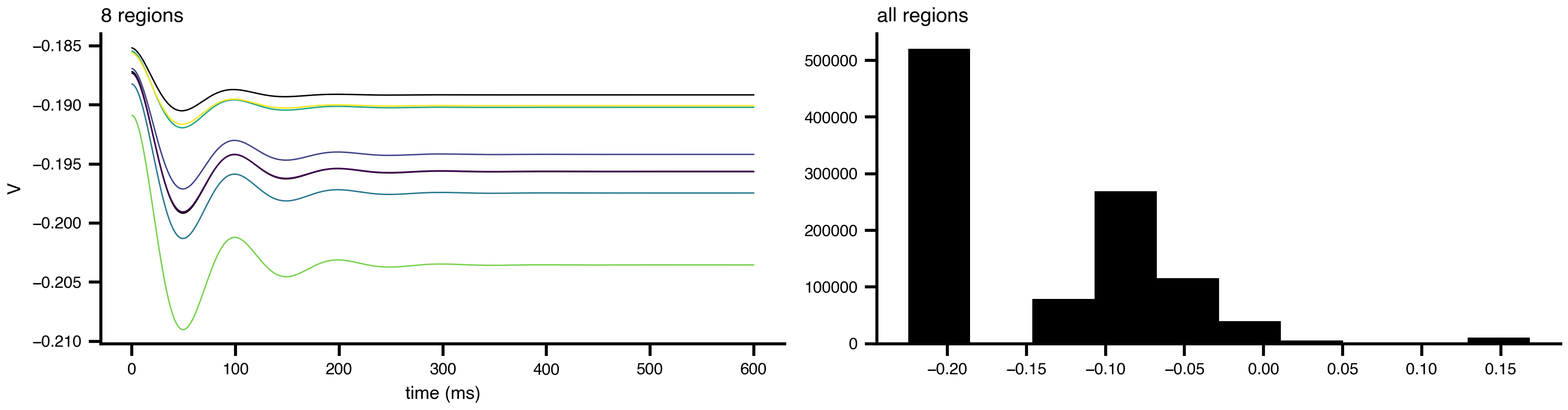

Figure 3: Eight of 87 regions, and the same simulation as a raster over all regions.

Two things that bite newcomers

Normalize the connectome. Connectomes are stored in native units: the Desikan-Killiany matrix holds streamline counts in the hundreds of thousands. Feeding those in raw makes the drive enormous and the run returns NaN. The transforms block above rescales so the mean non-zero weight is \(1\).
The coupling key is the model’s input port, here c_glob: not a name you invent. Get it from list(exp.dynamics.coupling_inputs).

Where to go next

The documentation follows the shape of an experiment — specify it, run it, then analyze the result:

You want to…	Go to
See the whole spec as one object	The SimulationExperiment object
Write or pick a model	Models & dynamics
Build or load a connectome	Networks & connectomes
Measure something (BOLD, FC, EEG)	Observation models
Sweep parameters	Parameter exploration
Match a model to data	Fitting, inference & optimization
Run on JAX, TVB, Julia, …	Run on a backend
Find where behaviour changes	Bifurcation & stability
Add spiking or multi-scale detail	Beyond the mean field
Scale up to a cluster	Reproducible workflows

New to the science itself? The natural reading order follows the field’s own arc: single-system dynamics and bifurcations → neuron and neural-mass models → whole-brain networks. Start with Models & dynamics, then Bifurcation & stability, then Networks & connectomes.

Coming from another tool? Interoperability maps TVBO onto TVB, PyRates, NeuroML, tvboptim, the Julia backends, BIDS and openMINDS.