Bayesian Inference of Stimulation & Excitability via tvboptim
Recover a pulse amplitude and a node’s excitability from one noisy recording, and watch the priors slide the posterior along the ridge where the two trade off.
A 1 ms pulse drives a single Generic2dOscillator node out of its quiescent state, and one noisy recording of \(V\) is all the evidence there is. Two unknowns produced it: the pulse amplitude and the node’s excitability\(I\). A weak pulse into an excitable node and a strong pulse into a quiet one leave almost the same trace, so the two are not separately identifiable from one recording, and a point estimate would report a number the data does not support. NUTS/MCMC reports the whole ridge instead, and the prior decides where on it the mass sits.
Everything below is declared in Bayesian_tvboptim.yaml and the curated experiment it references. The page runs that recipe and shows what it produced; it contains no plotting code and no analysis of its own.
The recipe
The study is one line, because the experiment is curated: it is referenced by IRI rather than copied, so this page and the database cannot drift apart.
The recording the inference is fitted to is an Observation like any other: the forward run at the true parameters, subsampled, plus Gaussian measurement noise at a fixed seed. Declaring it is what makes the three scenarios comparable: they are fitted to the same numbers, and those numbers come back from this recipe alone rather than from whatever the page happened to draw.
Each scenario then names that observation as the data its likelihood scores, and recorded_ts as what the model predicts, and differs from the others in nothing but the width of its priors. The two have to be named apart: the noise is one deterministic draw, so applying it to the prediction as well would put it on both sides of the residual and cancel it, leaving an inference that fits noiseless data while the recipe says otherwise.
SimulationStudy.run() executes the whole recipe in process (the forward run, the three samplers, then the figure they declare) and returns a StudyResult. It is the Python form of tvbo run Bayesian_tvboptim.yaml, on the same orchestration, so a notebook and the command line cannot disagree.
from tvbo import SimulationStudystudy = SimulationStudy.from_file("Bayesian_tvboptim.yaml")results = study.run(root="../../_build/Bayesian_tvboptim")results
* Owlready2 * Warning: ignoring cyclic subclass of/subproperty of, involving:
  http://uri.interlex.org/tgbugs/uris/readable/atlas/Space

INFO [tvbo.run] [+0s] STEP 1: Running simulation...
INFO [tvbo.run] [+1s]   Simulation period: 150.0 ms, dt: 0.2 ms
INFO [tvbo.run] [+1s]   Simulation complete.
INFO [tvbo.run] [+1s] STEP 5: Running Bayesian inference (MCMC)...
INFO [tvbo.run] [+14s]   Inference complete. Posteriors: ['scenario_A', 'scenario_B', 'scenario_C']
INFO [tvbo.run] [+14s] Experiment complete.
INFO [tvbo.cli] done: ExperimentResult
INFO [tvbo.cli] wrote ['/Users/leonmartin_bih/tools/tvbo/docs/_build/Bayesian_tvboptim/derivatives/tvbo/exp-8_model-Generic2dOscillator_result.h5', '/Users/leonmartin_bih/tools/tvbo/docs/_build/Bayesian_tvboptim/derivatives/tvbo/exp-8_model-Generic2dOscillator_result.yaml']
INFO [tvbo.cli] rendering 1 figure(s) -> /Users/leonmartin_bih/tools/tvbo/docs/_build/Bayesian_tvboptim/docs/figures
INFO [tvbo.cli] bayesian_recovery FAILED (KeyError: '{}')
WARNING [tvbo.cli] figure rendering failed (RuntimeError: 1 of 1 figures did not render:
  bayesian_recovery: KeyError: '{}'); the experiment results are saved. Re-run `tvbo figure render /Users/leonmartin_bih/tools/tvbo/docs/examples/fitting/Bayesian_tvboptim.yaml` to retry.
A posterior comes back where the recipe put it. inferences.scenario_A.posterior is the group the inferences: block declared, and its variables are the parameters named in priors:, spelled <component>.<parameter> as the recipe spells them. Every draw of both parameters sits on the same draw axis, which is what makes the joint plot below a scatter rather than an outer product.
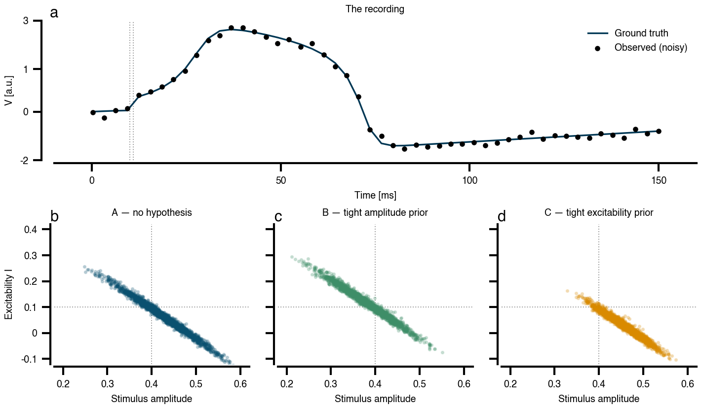
Bayesian recovery of stimulus amplitude and excitability. One noisy recording, three prior scenarios, and the degeneracy ridge that makes a point estimate misleading here. (a) The recording. line of time (integration__recorded_ts), scatter of time (integration__observed_ts) from experiment 8. The noiseless forward run at the true parameters (line) and the noisy recording the inference is given (points) — one trace, 50 samples. The rules mark the 1 ms pulse. (b) A — no hypothesis. scatter of inference__scenario_A__posterior__stimulus.amplitude (inference__scenario_A__posterior__Generic2dOscillator.I) from experiment 8. Wide priors on both parameters. The draws fall on a line, not in a blob: a weak pulse into an excitable node and a strong pulse into a quiet one fit this recording equally well, and one trace cannot separate them. The rules cross at the truth. (c) B — tight amplitude prior. scatter of inference__scenario_B__posterior__stimulus.amplitude (inference__scenario_B__posterior__Generic2dOscillator.I) from experiment 8. Pinning the amplitude does not shrink the posterior towards the truth: it slides along the same ridge, and the excitability takes up what the amplitude is no longer allowed to explain. (d) C — tight excitability prior. scatter of inference__scenario_C__posterior__stimulus.amplitude (inference__scenario_C__posterior__Generic2dOscillator.I) from experiment 8. The mirror image: pinning I moves the mass the other way along the ridge.
Under wide priors (b) the posterior recovers the truth: amplitude \(0.43 \pm 0.06\) against a true \(0.40\), excitability \(0.064 \pm 0.067\) against a true \(0.10\). But the two are correlated at \(-0.99\), so the cloud is a line, and its width along that line is the answer, not the marginal spread of either parameter on its own.
That is what makes (c) and (d) the point of the page. Tightening the amplitude prior (c) does not pull the posterior towards the truth; it slides it down the ridge, to amplitude \(0.38\) and excitability \(0.12\). Tightening the excitability prior instead (d) slides it the other way, to \(0.46\) and \(0.027\). Each is a confident, well-mixed posterior, with all three scenarios returning \(\hat{R} \approx 1.00\), and each is confident about a different place on the same ridge. The prior is doing the identifying that the recording cannot.
See also
Model fitting — how losses and gradients work in TVBO.