Sweep a model’s knobs and watch what the network does
Declare a grid of parameter values and run the cells in parallel to see how network behaviour changes across the sweep.
Part of the running example, where stage 4 adds an explorations grid over the drive.
A brain network model is a hypothesis with knobs. Choosing knob values is how the hypothesis gets tested, and before fitting anything it pays to know how the model behaves across its parameter range: where it is quiet, where it oscillates, and where it changes character.
An exploration evaluates \(\hat{y}(\theta)\) on a grid of \(\theta\) values. TVBO declares that grid in the same YAML as the model, evaluates the cells vectorized in parallel (see Parallelization), and returns the results as a labelled array indexed by the swept parameter.
Declaring a sweep
An explorations block names the sweep, lists the axes in space, and says how to combine them. Each axis is addressed as <scope>.<parameter>:
domain: {lo, hi, n} gives n evenly spaced values. mode: product takes the Cartesian product of the axes, so two axes of 9 and 5 points run 45 cells; mode: zip would pair them instead.
Running it
One run() executes the whole grid.
res = exp.run().explorations.g_sweepprint(res)print("axis:", res.axes[0].name, "->", res.axes[0].explored_values)
INFO [tvbo.run] [+0s] STEP 1: Running simulation...
INFO [tvbo.run] [+1s]   Simulation period: 400.0 ms, dt: 0.1 ms
INFO [tvbo.run] [+1s]   Transient period: 100.0 ms (settled on (-100.0, 0], warm-started via update_history)
INFO [tvbo.run] [+1s]   Simulation complete.
INFO [tvbo.run] [+1s] STEP 2: Running explorations...
INFO [tvbo.run] [+1s]   > g_sweep
INFO [tvbo.run]   grid batch 1/1 (100%)
INFO [tvbo.run] [+1s]   Explorations complete.
INFO [tvbo.run] [+1s] Experiment complete.
The result is indexed by the swept parameter. as_grid() returns a labelled array whose first dimension is the axis, so cells are selected by value rather than by position:
# The exploration grid leaves the state axis unlabelled; attach the model's own# state-variable names so selection stays keyed rather than positional.names =list(exp.dynamics.state_variables)grid = res.as_grid().assign_coords(variable=names)V = grid.sel(variable="V")print("dims:", dict(zip(V.dims, V.shape)))print("state order:", names)
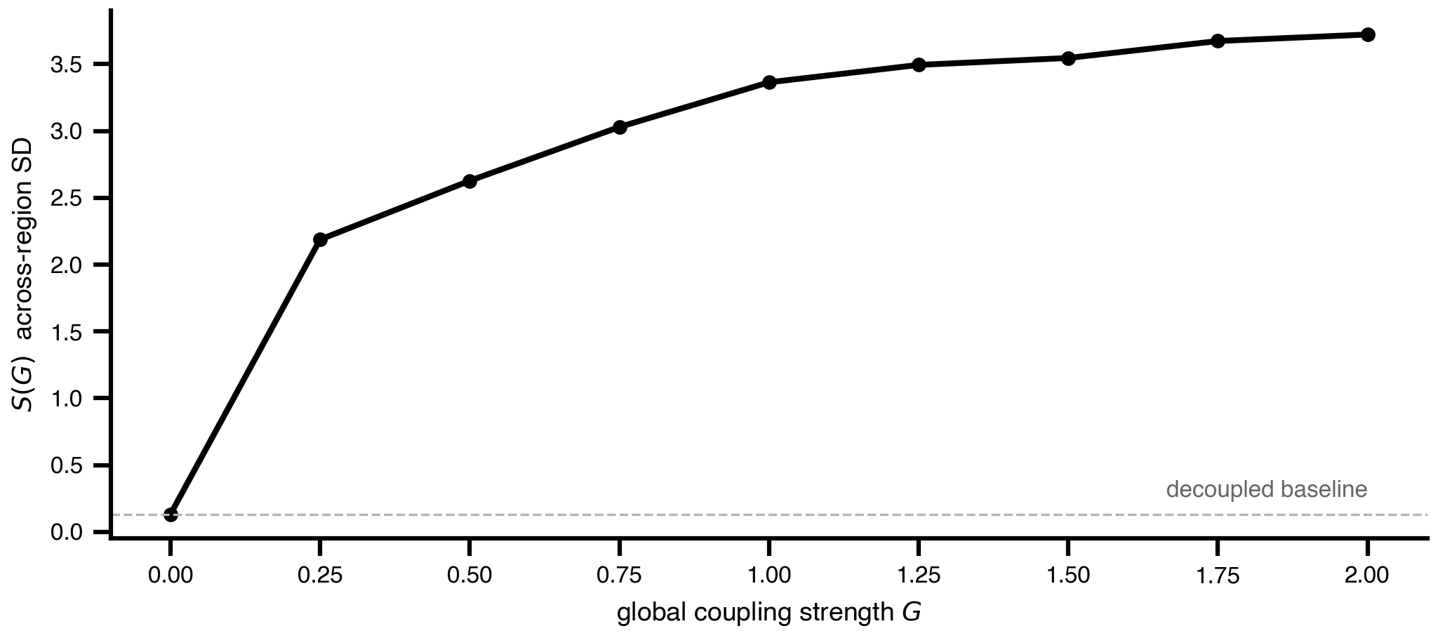
A sweep is only useful with a summary statistic that collapses each cell to a number. Here the question is whether regions keep their own identity, so the statistic is the standard deviation across regions, averaged over time:
Figure 1: Across-region variability against global coupling strength. The model jumps off the decoupled baseline as soon as coupling is switched on, then grows gradually.
The same numbers as a table
import pandas as pdpd.DataFrame({"G": np.round(Gs, 3), "across-region SD": np.round(S, 4)})
Table 1
G
across-region SD
0
0.00
0.1327
1
0.25
2.1877
2
0.50
2.6274
3
0.75
3.0297
4
1.00
3.3642
5
1.25
3.4942
6
1.50
3.5461
7
1.75
3.6730
8
2.00
3.7216
At \(G = 0\) the regions are effectively independent and \(S\) sits at its baseline. Switching coupling on moves the network off that baseline immediately, after which \(S\) grows steadily. The interesting region of a sweep is almost always where the curve bends, not where it is flat — that is where the model changes qualitative behaviour, and it is the natural place to look with bifurcation analysis.
Inspecting individual cells
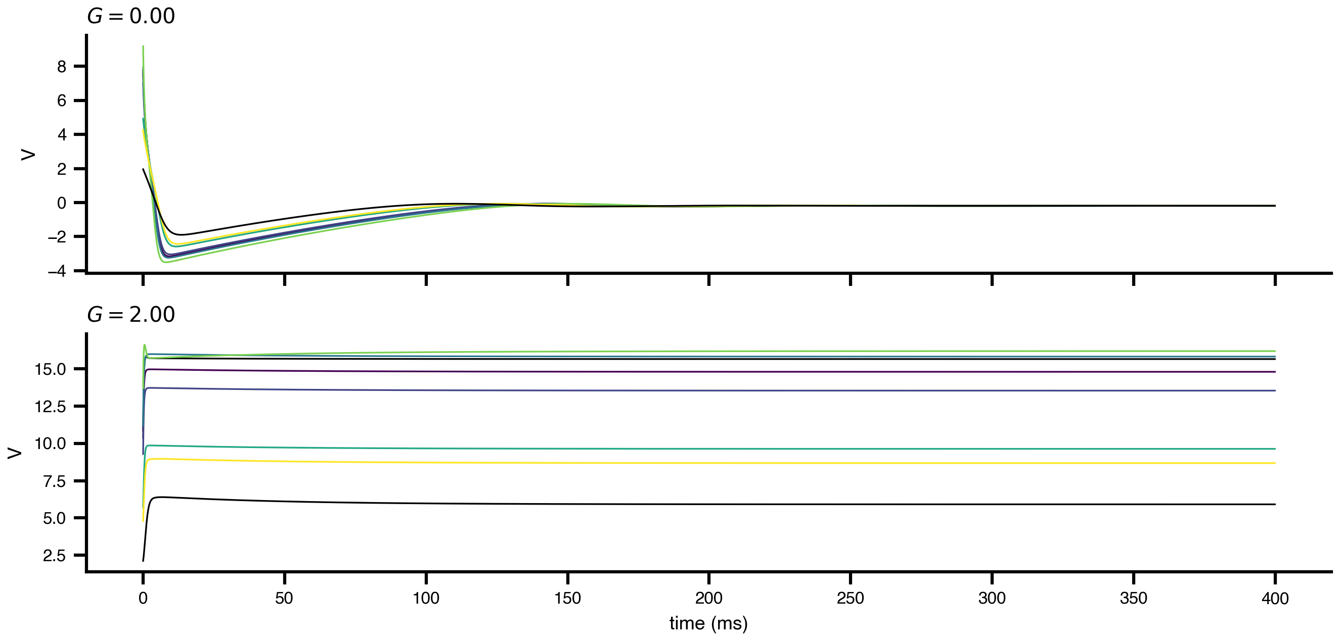
Because the grid is labelled, a single cell can be pulled out by its parameter value and plotted like any other simulation:
Code
fig, axes = plt.subplots(2, 1, figsize=(9, 4.4), sharex=True)for ax, g inzip(axes, [float(Gs[0]), float(Gs[-1])]): cell = V.sel({"c_glob.G": g}) # select by value, not index ax.plot(cell.time, cell.isel(node=slice(0, 8)), lw=0.8) ax.set_ylabel("V") ax.set_title(f"$G = {g:.2f}$", loc="left", fontsize=10)axes[-1].set_xlabel("time (ms)")plt.tight_layout()plt.show()
Figure 2: Eight regions at weak versus strong coupling, selected from the grid by parameter value.
Several axes at once
Axes compose. Sweeping coupling strength against conduction speed explores how delays and drive interact, on a grid of \(9 \times 5 = 45\) cells:
network.conduction_speed is special: changing it rebuilds the delay graph for every cell, so the sweep genuinely re-derives \(\tau_{ij} = L_{ij}/v\) rather than reusing one set of delays.
A network whose edges carry an explicit delay instead of a tract length sweeps that delay directly, with network.edges.delay. The two are alternatives, not a choice of style: a connectome that measures tract lengths derives its delays from the conduction speed, so it is the speed that is sweepable there, and TVBO says so rather than sweeping nothing. Either way the history buffer is sized once, before compilation, for the longest delay the sweep can reach.
Parallelization
Grid cells are independent simulations, so TVBO evaluates them vectorized: one compiled kernel steps a batch of cells at once with jax.vmap, far faster than looping cell by cell. The batch width is n_parallel, and it defaults to auto:
explorations:my_sweep:space:{ ... }n_parallel: auto # the default — you rarely need to set it
auto vectorizes the grid, bounded two ways: a cell-count cap (min(grid_size, 64), past the point where per-cell throughput saturates, so it keeps the full speed-up) and a memory budget (default 2 GB). Vectorizing holds n_vmap cells’ working state at once — so auto does use more memory than a sequential run — and the budget, sized against the per-cell output and live state, keeps that from ballooning on a large-per-cell grid such as a whole-brain delay network. On a big-memory machine, raise the count cap with TVBO_NVMAP_AUTO_CAP or the budget with TVBO_NVMAP_MEM_BUDGET_GB (both are portable defaults, not hardware limits).
An integer fixes the chunk width and bypasses both bounds. n_parallel: 1 is fully sequential (slowest, smallest footprint); a larger value like 256 packs wider batches (fewer kernel launches, more working memory) and only helps on a very large grid with memory to spare.
The result array, grid_size × timepoints × …, is materialized in full regardless of n_parallel; for a full-trajectory sweep that, not the batch width, is what bounds a grid on one machine.
Grids grow fast
mode: product multiplies. Three axes of 10 points is 1000 simulations. Start coarse, find the interesting region, then refine — and move large grids to a cluster with tvbo workflow and the HPC patterns rather than running them locally.
Where to go next
Found an interesting region?Bifurcation analysis characterizes what changes there, instead of only where.
Want the best parameters, not the landscape?Fitting, inference & optimization optimizes \(\theta\) against data rather than enumerating it.