3. Saddle-Node

The saddle-node (also “fold” or “tangent”) bifurcation is the simplest codimension-1 local bifurcation:

\[ \dot x = a - x^2. \]

For \(a < 0\): no real equilibrium, \(\dot x < 0\) everywhere — every trajectory escapes to \(-\infty\).
For \(a = 0\): a single non-hyperbolic fixed point at \(x = 0\), \(f'(0) = 0\).
For \(a > 0\): two fixed points \(x_{\pm} = \pm\sqrt a\), the upper one stable (\(f'(x_+) = -2\sqrt a < 0\)), the lower one unstable.

The two equilibria collide and annihilate at \(a = 0\) — the codim-1 saddle-node bifurcation. Beyond it, the system has no attractors at all in this neighbourhood.

from tvbo import Dynamics, Continuation, SimulationExperiment

SN_YAML = """
name: SaddleNode
description: Canonical saddle-node $\\dot x = a - x^2$.
parameters:
  a:
    name: a
    value: 1.0
state_variables:
  x:
    name: x
    domain: { lo: -2.0, hi: 2.0 }
    equation:
      lhs: Derivative(x, t)
      rhs: a - x**2
    initial_value: 1.0
"""

CONT_YAML = """
name: sn_in_a
dynamics: SaddleNode
free_parameters:
  - name: a
    domain: { lo: -2.0, hi: 2.0 }
max_steps: 200
ds: 0.01
bothside: true
"""

dyn = Dynamics.from_string(SN_YAML)
cont = Continuation.from_string(CONT_YAML)
exp = SimulationExperiment(dynamics=dyn, continuations=[cont])

Phase line \(f(x)\) across the bifurcation

For a 1-D ODE, the phase line is just the graph of \(f(x) = a - x^2\) with arrows showing the sign of \(\dot x\). As \(a\) increases through \(0\), the parabola lifts above the \(x\)-axis and two equilibria are born from a single tangency point.

import numpy as np
import matplotlib.pyplot as plt

x = np.linspace(-2, 2, 400)
fig, axes = plt.subplots(1, 3, figsize=(12, 3.6), sharey=True)
for ax, a in zip(axes, [-0.5, 0.0, 0.5]):
    f = a - x**2
    ax.axhline(0, color="0.7", lw=0.8)
    ax.plot(x, f, lw=2, color="C0")
    roots = np.roots([-1, 0, a])
    for r in roots[np.isreal(roots)].real:
        slope = -2*r
        ax.plot(r, 0, "o", color="tab:green" if slope < 0 else "tab:red", ms=8, mec="k")
    ax.set_xlim(-2, 2); ax.set_ylim(-2.5, 1.0)
    ax.set_xlabel("$x$"); ax.set_title(f"$a = {a}$")
axes[0].set_ylabel(r"$\dot x = a - x^2$")
plt.tight_layout(); plt.show()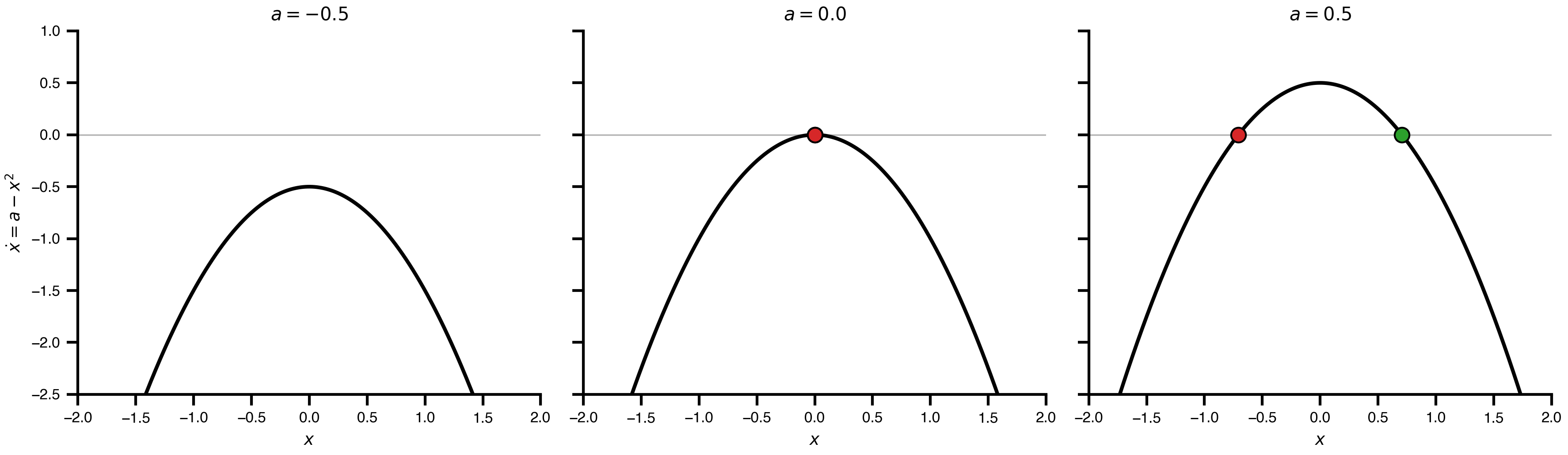

Green = stable, red = unstable. At \(a = 0\) the two markers merge into a single half-stable point (tangent to the \(x\)-axis).

BifurcationKit.jl

result_jl = exp.run("bifurcationkit.jl")
result_jl.continuations["sn_in_a"].plot(VOI="x")
plt.gca().set_xlim(-2, 2); plt.gca().set_ylim(-2, 2); plt.show()

Detected IPython. Loading juliacall extension. See https://juliapy.github.io/PythonCall.jl/stable/compat/#IPython
CT: 1.274568 seconds (3.31 M allocations: 165.707 MiB, 17.24% gc time, 99.80% compilation time)
CT: 0.000417 seconds (7.60 k allocations: 318.734 KiB)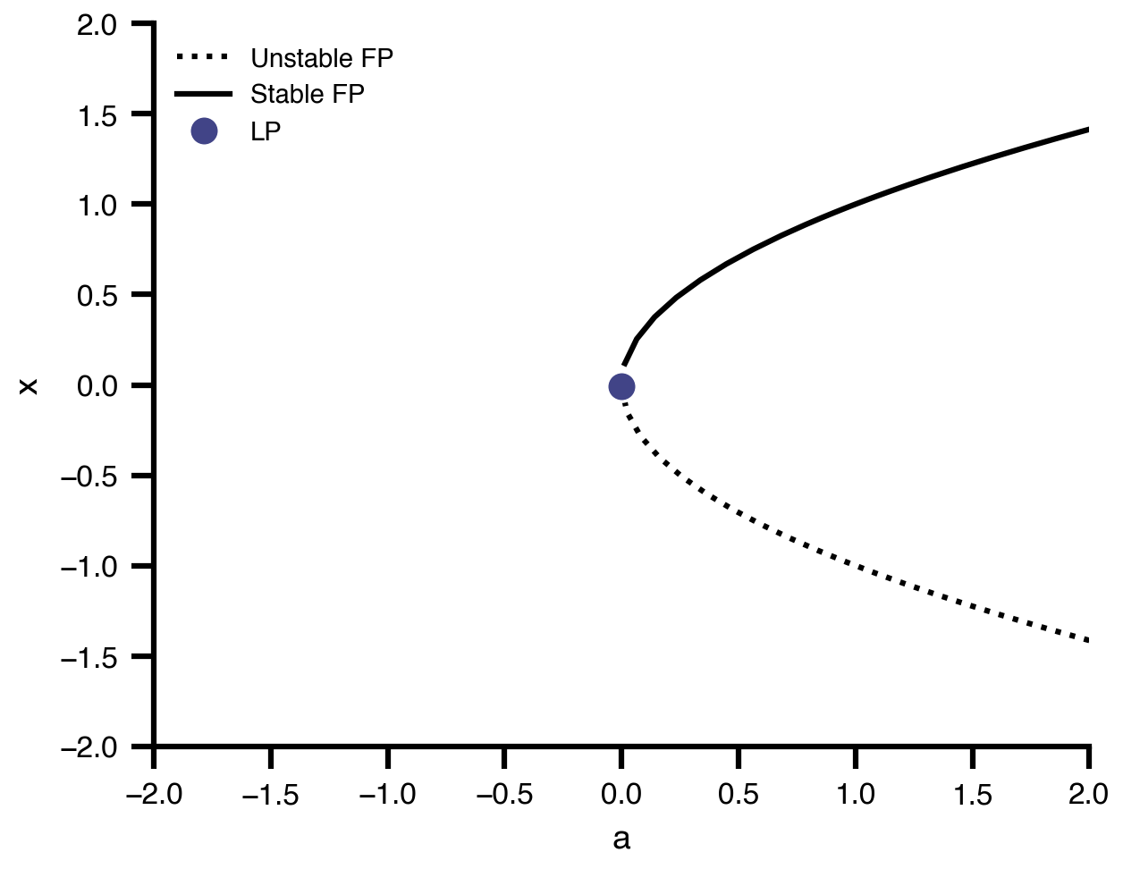

PyRates / PyCoBi

PyRates itself can represent the 1-D system fine, and AUTO-07p continues it without trouble — but PyCoBi’s summary builder requires NDIM >= 2 and raises KeyError('U(1)') on scalar ODEs. The adapter detects this and raises a clear NotImplementedError:

try:
    result_py = exp.run("pyrates-bifurcation")
    result_py.continuations["sn_in_a"].plot(VOI="x")
except NotImplementedError as e:
    print(e)

Compilation Progress
--------------------
    (1) Translating the circuit template into a networkx graph representation...
        ...finished.
    (2) Preprocessing edge transmission operations...
        ...finished.
    (3) Parsing the model equations into a compute graph...
        ...finished.
    Model compilation was finished.
The 'pyrates-bifurcation' backend cannot continue the 1-D system 'SaddleNode' (state variables: ['x']). PyCoBi's summary builder requires NDIM >= 2 and raises KeyError('U(1)') for scalar ODEs. For 1-D systems use the 'auto-07p' or 'bifurcationkit.jl' backend instead.

For 1-D toy systems use auto-07p (below) or bifurcationkit.jl.

AUTO-07p (NumCont)

This is the backend used by the original standalone SaddleNode.py example: an AUTO-07p Fortran binary built on-the-fly from the YAML, then continued bidirectionally (bothside: true ↔︎ standalone DS=-0.01).

result_auto = exp.run("auto-07p")
result_auto.continuations["sn_in_a"].plot(VOI="x")
plt.gca().set_xlim(-2, 2); plt.gca().set_ylim(-2, 2); plt.show()

/opt/homebrew/bin/gfortran -arch arm64 -O -fopenmp -O -c /var/folders/ym/9kw1g21j1nd7kwfn8c0z3st40000gn/T/tvbo_numcont_SaddleNode_v1wj62ij/model.f90 -o /var/folders/ym/9kw1g21j1nd7kwfn8c0z3st40000gn/T/tvbo_numcont_SaddleNode_v1wj62ij/model.o
/opt/homebrew/bin/gfortran -arch arm64 -O -fopenmp -O /var/folders/ym/9kw1g21j1nd7kwfn8c0z3st40000gn/T/tvbo_numcont_SaddleNode_v1wj62ij/model.o -o /var/folders/ym/9kw1g21j1nd7kwfn8c0z3st40000gn/T/tvbo_numcont_SaddleNode_v1wj62ij/model.exe /Applications/auto-07p/lib/*.o
Starting /var/folders/ym/9kw1g21j1nd7kwfn8c0z3st40000gn/T/tvbo_numcont_SaddleNode_v1wj62ij/model ...

ld: warning: duplicate -rpath '/Library/Developer/CommandLineTools/SDKs/MacOSX26.4.sdk/usr/lib' ignored


  BR    PT  TY  LAB       a          L2-NORM          x       
   1     1  EP    1   1.00000E+00   1.00000E+00   1.00000E+00
   1    10        2   1.20109E+00   1.09594E+00   1.09594E+00
   1    20        3   1.55022E+00   1.24508E+00   1.24508E+00
   1    30  EP    4   2.04811E+00   1.43112E+00   1.43112E+00

 Total Time    0.165E-02
/var/folders/ym/9kw1g21j1nd7kwfn8c0z3st40000gn/T/tvbo_numcont_SaddleNode_v1wj62ij/model ... done
Starting /var/folders/ym/9kw1g21j1nd7kwfn8c0z3st40000gn/T/tvbo_numcont_SaddleNode_v1wj62ij/model ...

  BR    PT  TY  LAB       a          L2-NORM          x       
   1     1  EP    1   1.00000E+00   1.00000E+00   1.00000E+00
   1    10        2   8.02934E-01   8.96066E-01   8.96066E-01
   1    20        3   4.81697E-01   6.94044E-01   6.94044E-01
   1    30        4   1.97049E-01   4.43902E-01   4.43902E-01
   1    40        5   1.34522E-02   1.15984E-01   1.15984E-01
   1    44  LP    6  -2.74675E-17   3.53563E-09  -3.53563E-09
   1    50        7   4.87844E-02   2.20872E-01  -2.20872E-01
   1    60        8   2.74087E-01   5.23533E-01  -5.23533E-01
   1    70        9   5.72943E-01   7.56930E-01  -7.56930E-01
   1    80       10   9.00364E-01   9.48875E-01  -9.48875E-01
   1    90       11   1.24198E+00   1.11444E+00  -1.11444E+00
   1   100       12   1.59191E+00   1.26171E+00  -1.26171E+00
   1   108  EP   13   2.00091E+00   1.41453E+00  -1.41453E+00

 Total Time    0.135E-02
/var/folders/ym/9kw1g21j1nd7kwfn8c0z3st40000gn/T/tvbo_numcont_SaddleNode_v1wj62ij/model ... done
Merge done
Saving to sn_in_a, sn_in_a, and sn_in_a ... done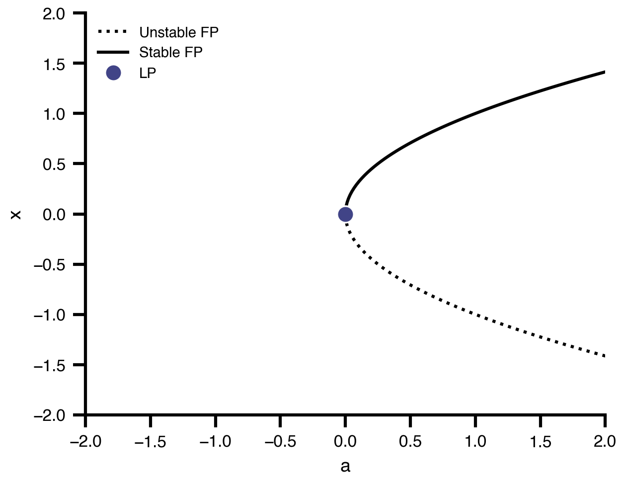

The fold point appears at \(a = 0\) in all three backends. The upper branch is stable, the lower branch unstable. Beyond the fold the equilibria simply disappear — there is no continuous deformation back; only a topological change. This is the prototype for regime shifts in nonlinear systems.