from tvbo import Dynamics
import matplotlib.pyplot as plt

CASES = {
    "Saddle":       ("x1 - x2",  "-x1 - x2"),       # tr=0, det=-2
    "Stable node":  ("-2*x1",    "-x2"),            # tr=-3, det=2
    "Stable focus": ("-0.3*x1 - x2",  "x1 - 0.3*x2"),  # tr=-0.6, det=1.09
    "Centre":       ("-x2",      "x1"),             # tr=0, det=1
}

def make_yaml(rhs1, rhs2, name):
    return f"""
name: {name}
state_variables:
  x1:
    name: x1
    domain: {{ lo: -2.0, hi: 2.0 }}
    equation:
      lhs: Derivative(x1, t)
      rhs: {rhs1}
    initial_value: 1.0
  x2:
    name: x2
    domain: {{ lo: -2.0, hi: 2.0 }}
    equation:
      lhs: Derivative(x2, t)
      rhs: {rhs2}
    initial_value: 1.0
"""2. 2D Phase Portraits
For two-dimensional linear systems
\[ \dot{\vec x} = A\,\vec x, \qquad A = \begin{pmatrix} a_{11} & a_{12} \\ a_{21} & a_{22} \end{pmatrix} \]
the eigenvalues \(\lambda_{1,2}\) of \(A\) fully classify the equilibrium at the origin. The four canonical cases:
| Case | Trace\((A)\) | Det\((A)\) | Eigenvalues | Phase portrait |
|---|---|---|---|---|
| Stable node | \(< 0\) | \(> 0\), \(\Delta > 0\) | \(\lambda_{1,2} \in \mathbb{R}_{<0}\) | trajectories converge tangent to slow manifold |
| Saddle | any | \(< 0\) | \(\lambda_1 \lambda_2 < 0\) | crossing stable / unstable manifolds |
| Stable focus | \(< 0\) | \(> 0\), \(\Delta < 0\) | \(\alpha \pm i\omega,\;\alpha < 0\) | inward spiral |
| Centre | \(= 0\) | \(> 0\) | \(\pm\,i\omega\) | nested closed orbits |
with \(\Delta = (\mathrm{tr}\,A)^2 - 4\det A\). We sweep all four cases with identical plotting code: only the rhs strings change.
Phase planes for the four canonical cases
Each panel uses the new kind='phaseplane' shortcut, which overlays the vector field with the two nullclines (\(\dot x_1 = 0\) in blue, \(\dot x_2 = 0\) in red) and marks the fixed points detected on the grid (black circles). Axis limits are set declaratively via the YAML domain.lo / hi.
fig, axes = plt.subplots(2, 2, figsize=(9, 8))
for ax, (label, (r1, r2)) in zip(axes.flat, CASES.items()):
    dyn = Dynamics.from_string(make_yaml(r1, r2, label.replace(" ", "")))
    dyn.plot("x1", "x2", kind="phaseplane", ax=ax,
             grid_n=22, n_trajectories=3, duration=15)
    ax.set_title(label)
plt.tight_layout(); plt.show()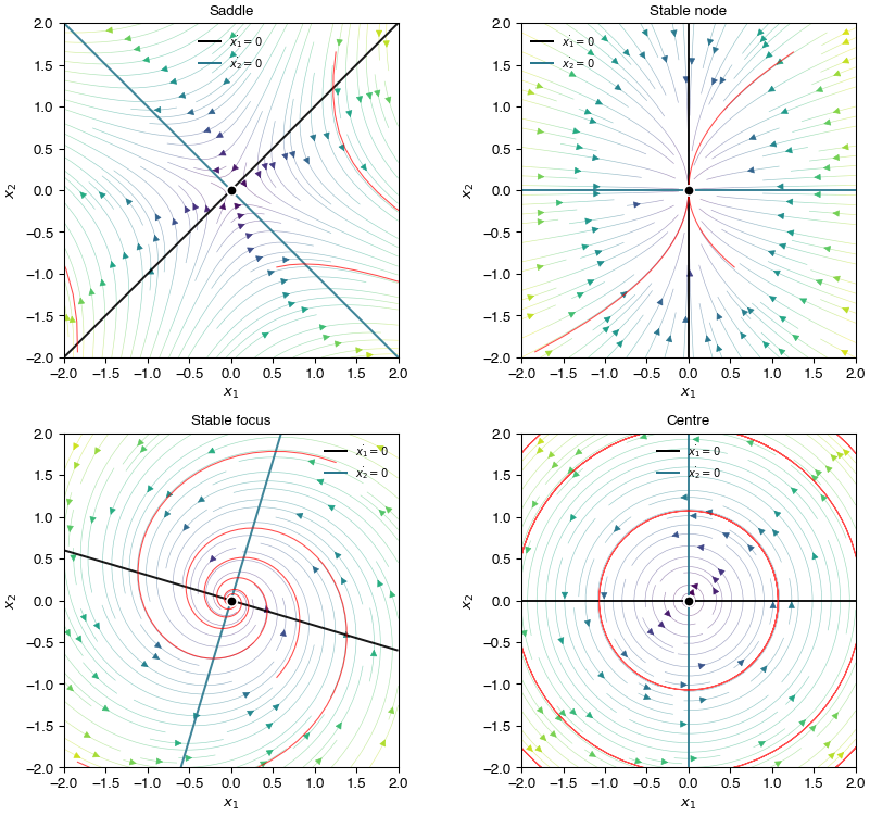
Saddle case in isolation (PhasePortraitSaddle.png)
The legacy figure focuses on the saddle with \(A = \begin{pmatrix} 1 & -1 \\ -1 & -1 \end{pmatrix}\), \(\lambda_{\pm} = \pm\sqrt 2\):
dyn = Dynamics.from_string(make_yaml("x1 - x2", "-x1 - x2", "Saddle2D"))
dyn.plot("x1", "x2", kind="phaseplane", n_trajectories=4, duration=10)
plt.gca().set_xlim(-2, 2); plt.gca().set_ylim(-2, 2)
plt.show()
The two orthogonal nullclines intersect only at the origin, where the saddle sits. Trajectories are pulled along the stable manifold and ejected along the unstable one.
Linking to nonlinear bifurcations
A nonlinear vector field \(\dot{\vec x} = f(\vec x)\) can have many equilibria. Linearisation at each one gives a 2D matrix \(A = Df(\vec x^*)\) that classifies its local topology using the table above. Bifurcations occur when the eigenvalues of one of those matrices crosses the imaginary axis as a parameter varies — the topic of the rest of this tutorial.