# =============================================================================
# Cascading Failure in a Power Grid
# =============================================================================
# Source: https://juliadynamics.github.io/NetworkDynamics.jl/stable/generated/cascading_failure/
#
# Swing equation power grid model with component-based callbacks for
# line tripping. Demonstrates:
#   - find_fixpoint for initial conditions
#   - ContinuousComponentCallback for threshold-triggered line failure
#   - PresetTimeComponentCallback for initial perturbation
#
# Reference: Schäfer et al. (2018). Dynamically induced cascading failures
# in power grids. Nature Communications, 9(1), 1-13.
# =============================================================================

id: 105
label: "Cascading Failure"
description: >
    Minimal example of dynamic cascading failure in a power grid.
    Swing equation vertices with active power flow on edges. When the
    power flow on a line exceeds its limit, the line trips (K → 0).
    Uses find_fixpoint for steady-state initial conditions and
    component-based callbacks for discrete events.
    Recreates the NetworkDynamics.jl Cascading Failure tutorial.
references:
    - "https://juliadynamics.github.io/NetworkDynamics.jl/stable/generated/cascading_failure/"
    - "Schäfer, B., Witthaut, D., Timme, M., & Latora, V. (2018). Dynamically induced cascading failures in power grids. Nature Communications, 9(1), 1-13."

# -- Local Dynamics ------------------------------------------------------------
dynamics:
    name: SwingEquation
    label: "Swing equation"
    description: >
        Power grid node modeled by the swing equation.
        dδ/dt = ω, dω/dt = (P_ref - γ·ω + esum) / I.
        Output is the voltage angle δ (first state), used by edges for
        power flow computation.
    system_type: continuous
    autonomous: true
    parameters:
        P_ref:
            label: "Reference power"
            symbol: "P_ref"
            value: 0.0
            unit: "p.u."
            description: "Power setpoint: positive = generator, negative = load"
        I:
            label: "Inertia"
            symbol: "I"
            value: 1.0
            unit: "s²"
            description: "Rotational inertia of the generator/load"
        gamma:
            label: "Damping coefficient"
            symbol: "γ"
            value: 0.1
            unit: "1/s"
            description: "Droop / damping coefficient"
    coupling_terms:
        c_power:
            description: "Aggregated active power flow from incident edges"
    state_variables:
        delta:
            label: "Voltage angle"
            symbol: "δ"
            equation:
                rhs: "omega"
            initial_value: 0.0
            unit: "rad"
            coupling_variable: true
            variable_of_interest: true
        omega:
            label: "Angular velocity deviation"
            symbol: "ω"
            equation:
                rhs: "(P_ref - gamma * omega + c_power) / I"
            initial_value: 0.0
            unit: "rad/s"
            variable_of_interest: true

# -- Network -------------------------------------------------------------------
network:
    label: "5-node power grid"
    description: >
        Simple undirected graph with 5 nodes and 7 edges. Two generators
        (nodes 2, 5) and three loads (nodes 1, 3, 4).
    number_of_nodes: 5
    edges:
        # 7 undirected edges from adjacency matrix:
        # [0,1,1,0,1; 1,0,1,1,0; 1,1,0,1,0; 0,1,1,0,1; 1,0,0,1,0]
        - source: 0
          target: 1
        - source: 0
          target: 2
        - source: 0
          target: 4
        - source: 1
          target: 2
        - source: 1
          target: 3
        - source: 2
          target: 3
        - source: 3
          target: 4

    nodes:
        - id: 0
          label: "Load 1"
          parameters:
              - name: P_ref
                value: -1.0
        - id: 1
          label: "Generator 1"
          parameters:
              - name: P_ref
                value: 1.5
        - id: 2
          label: "Load 2"
          parameters:
              - name: P_ref
                value: -1.0
        - id: 3
          label: "Load 3"
          parameters:
              - name: P_ref
                value: -1.0
        - id: 4
          label: "Generator 2"
          parameters:
              - name: P_ref
                value: 1.5

    coupling:
        ActivePower:
            name: ActivePower
            label: "Active power flow"
            description: >
                Antisymmetric active power line: P = K sin(δ_src - δ_dst).
                Has additional parameter 'limit' for callback threshold.
            delayed: false
            parameters:
                K:
                    label: "Coupling strength"
                    value: 1.63
                    unit: "p.u."
                    description: "Line susceptance / coupling constant"
                limit:
                    label: "Line power limit"
                    value: 1.0
                    unit: "p.u."
                    description: "Threshold for line tripping"
            pre_expression:
                rhs: "K * sin(x_j - x_i)"
                description: "Active power flow"
            outsym:
                - P

# -- Events (callbacks) -------------------------------------------------------
events:
    edge_trip:
        event_type: continuous
        condition:
            rhs: "abs(u[:P]) - p[:limit]"
            description: "Triggers when power flow exceeds line limit"
        condition_states:
            - P
        condition_parameters:
            - limit
        affect:
            rhs: "p[:K] = 0"
            description: "Trip the line by setting coupling to zero"
        affect_parameters:
            - K
        target_component: all_edges

    initial_perturbation:
        event_type: preset_time
        trigger_times:
            - 1.0
        affect:
            rhs: "p[:K] = 0"
            description: "Trip line 5 at t=1.0 to start cascade"
        affect_parameters:
            - K
        target_component: "edge_5"

# -- Execution -----------------------------------------------------------------
execution:
    find_fixpoint: true

# -- Integration ---------------------------------------------------------------
integration:
    description: "Explicit Runge-Kutta (Tsit5) with dt=0.01 over t in [0, 6]"
    method: Tsit5
    step_size: 0.01
    duration: 6.0
    time_scale: "s"
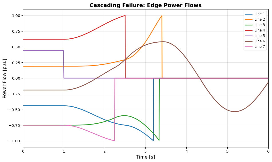
Cascading Failure
Dynamic line tripping in a power grid with component callbacks
Replicates the NetworkDynamics.jl Cascading Failure tutorial — swing equation power grid with dynamic line tripping. When power flow on a line exceeds its limit, the line is disconnected (K → 0), potentially triggering a cascade. Uses find_fixpoint for steady-state initial conditions and component-based callbacks for discrete events.
Reference: Schäfer, B., Witthaut, D., Timme, M., & Latora, V. (2018). Dynamically induced cascading failures in power grids. Nature Communications, 9(1), 1–13.
YAML Specification
Model Report
Cascading Failure
Minimal example of dynamic cascading failure in a power grid. Swing equation vertices with active power flow on edges. When the power flow on a line exceeds its limit, the line trips (K → 0). Uses find_fixpoint for steady-state initial conditions and component-based callbacks for discrete events. Recreates the NetworkDynamics.jl Cascading Failure tutorial.
1. Brain Network: 5-node power grid
Simple undirected graph with 5 nodes and 7 edges. Two generators (nodes 2, 5) and three loads (nodes 1, 3, 4).
- Regions: 5
Coupling: Active power flow
Antisymmetric active power line: P = K sin(δ_src - δ_dst). Has additional parameter ‘limit’ for callback threshold.
Receives \(\delta\) from connected regions.
Pre-synaptic: \(c_{\text{pre}} = - K \cdot \sin{\left(x_{i} - x_{j} \right)}\)
| Parameter | Value | Description |
|---|---|---|
| \(K\) | 1.63 | Line susceptance / coupling constant |
| \(limit\) | 1.0 | Threshold for line tripping |
2. Local Dynamics: Swing equation
Power grid node modeled by the swing equation. The model comprises 2 state variables.
2.1 State Equations
\[\dot{\delta} = \omega\]
\[\dot{\omega} = \frac{P_{ref} + c_{power} - \gamma \cdot \omega}{I}\]
2.2 Parameters
| Parameter | Value | Unit | Description |
|---|---|---|---|
| \(I\) | 1.0 | s2 | Rotational inertia of the generator/load |
| \(P_{ref}\) | 0.0 | per_unit | Power setpoint: positive = generator, negative = load |
| \(\gamma\) | 0.1 | per_s | Droop / damping coefficient |
3. Numerical Integration
- Method: Tsit5
- Time step: \(\Delta t = 0.01\) ms
- Duration: 6.0 ms
4. Execution
| Setting | Value |
|---|---|
| Workers | 1 |
| Precision | float64 |
| Random seed | 42 |
References
- https://juliadynamics.github.io/NetworkDynamics.jl/stable/generated/cascading_failure/
- Schäfer, B., Witthaut, D., Timme, M., & Latora, V. (2018). Dynamically induced cascading failures in power grids. Nature Communications, 9(1), 1-13.
Generated Julia Code
from tvbo import SimulationExperiment
exp = SimulationExperiment.from_file("yaml/cascading_failure.yaml")
Code(exp.render_code("networkdynamics"), language='julia')
using Graphs
using NetworkDynamics
using OrdinaryDiffEqTsit5
function SwingEquation_f!(dx, x, esum, (I, P_ref, gamma,), t)
delta, omega = x
c_power = esum[1]
dx[1] = omega
dx[2] = (P_ref + c_power - gamma .* omega) ./ I
nothing
end
vertex_SwingEquation = VertexModel(;
f = SwingEquation_f!,
g = StateMask(1:1),
sym = [:delta, :omega],
psym = [:I => 1.0, :P_ref => 0.0, :gamma => 0.1],
name = :SwingEquation,
)
function ActivePower_edge_g!(e_dst, v_src, v_dst, (K, limit,), t)
e_dst[1] = -K .* sin(v_dst[1] - v_src[1])
nothing
end
edge_ActivePower = EdgeModel(;
g = AntiSymmetric(ActivePower_edge_g!),
outsym = [:P],
psym = [:K => 1.63, :limit => 1.0],
name = :ActivePower,
)
g = SimpleGraph(5)
add_edge!(g, 1, 2)
add_edge!(g, 1, 3)
add_edge!(g, 1, 5)
add_edge!(g, 2, 3)
add_edge!(g, 2, 4)
add_edge!(g, 3, 4)
add_edge!(g, 4, 5)
nw = Network(g, vertex_SwingEquation, edge_ActivePower; dealias=true)
set_default!(nw, VIndex(1, :P_ref), -1.0)
set_default!(nw, VIndex(2, :P_ref), 1.5)
set_default!(nw, VIndex(3, :P_ref), -1.0)
set_default!(nw, VIndex(4, :P_ref), -1.0)
set_default!(nw, VIndex(5, :P_ref), 1.5)
u0 = find_fixpoint(nw)
set_defaults!(nw, u0)
s = NWState(nw)
edge_trip_cond = ComponentCondition([:P], [:limit]) do u, p, t
abs(u[:P]) - p[:limit]
end
edge_trip_affect = ComponentAffect([], [:K]) do u, p, ctx
p[:K] = 0
end
edge_trip_cb = ContinuousComponentCallback(edge_trip_cond, edge_trip_affect)
for i in 1:ne(g)
set_callback!(nw[EIndex(i)], edge_trip_cb)
end
initial_perturbation_cb = PresetTimeComponentCallback(1.0, edge_trip_affect)
add_callback!(nw[EIndex(5)], initial_perturbation_cb)
tspan = (0.0, 6.0)
u0 = NWState(nw)
prob = ODEProblem(nw, u0, tspan)
sol = solve(prob, Tsit5(); saveat=0.01)
adj_matrix = Float64.(adjacency_matrix(g))
using Random: MersenneTwister
function spring_layout(g; seed=42, iterations=50, k=1.0)
rng = MersenneTwister(seed)
n = nv(g)
pos = randn(rng, n, 2)
for _ in 1:iterations
disp = zeros(n, 2)
for i in 1:n, j in (i+1):n
d = pos[i, :] - pos[j, :]
dist = max(norm(d), 0.01)
rep = k^2 / dist
disp[i, :] .+= d / dist * rep
disp[j, :] .-= d / dist * rep
end
for e in edges(g)
i, j = src(e), dst(e)
d = pos[j, :] - pos[i, :]
dist = max(norm(d), 0.01)
att = dist^2 / k
disp[i, :] .+= d / dist * att
disp[j, :] .-= d / dist * att
end
for i in 1:n
dl = max(norm(disp[i, :]), 0.01)
pos[i, :] .+= disp[i, :] / dl * min(dl, 0.1)
end
end
return pos
end
using LinearAlgebra: norm
node_positions = spring_layout(g)
using Plots
plot(sol; ylabel="state", xlabel="time", title="SwingEquation on 5-node network")
Run & Plot
import numpy as np
import matplotlib.pyplot as plt

# Run simulation — edge observables extracted automatically from outsym metadata
ts = exp.run(format="networkdynamics")
power_flows = ts.edge_data['P']

# Plot edge power flows (matches ND.jl tutorial)
fig, ax = plt.subplots(figsize=(10, 6))
for i in range(power_flows.shape[1]):
    ax.plot(ts.time, power_flows[:, i], label=f'Line {i+1}', lw=2)

ax.set_xlabel('Time [s]', fontsize=12)
ax.set_ylabel('Power Flow [p.u.]', fontsize=12)
ax.set_title('Cascading Failure: Edge Power Flows', fontsize=14, fontweight='bold')
ax.legend(loc='best', fontsize=9)
ax.grid(True, alpha=0.3)
ax.set_xlim(0, 6)
plt.tight_layout()
plt.show()
Detected IPython. Loading juliacall extension. See https://juliapy.github.io/PythonCall.jl/stable/compat/#IPython