The running example

One Jansen-Rit experiment, grown one block at a time

A single experiment that starts as one cortical column and ends as a drive sweep on a connectome — each block linked to the page that documents it.

Every page in ② SPECIFY documents one block of a specification, and each stands on its own snippet so you can read it in isolation. This page is the thread that connects them: one experiment, grown six times, where each growth step is exactly the block one of those pages is about.

The model is Jansen-Rit, the cortical column whose rhythm depends on how hard it is driven. Every number below is computed when this page is built, so the claims are whatever the code actually produces.

Imports, plot style, and a spectrum helper

import warnings; warnings.filterwarnings("ignore")
import numpy as np
import matplotlib.pyplot as plt
import bsplot
from tvbo import SimulationExperiment

bsplot.style.use("tvbo")

DT = 0.5  # ms, the step size every stage below integrates at

def spectrum(x):
    """Return (frequencies, node-averaged power) for a time-by-node array."""
    x = np.asarray(x).squeeze()
    x = x[:, None] if x.ndim == 1 else x
    freqs = np.fft.rfftfreq(x.shape[0], d=DT / 1000.0)
    power = (np.abs(np.fft.rfft(x - x.mean(0), axis=0)) ** 2).mean(1)
    return freqs, power

def peak_hz(x, lo=1.0, hi=40.0):
    freqs, power = spectrum(x)
    band = (freqs > lo) & (freqs < hi)
    return float(freqs[band][power[band].argmax()])

def grow(spec, old, new):
    """Swap one block for another, refusing to pass a stale spec through silently."""
    if old not in spec:
        raise AssertionError(f"block not found in the previous stage:\n{old}")
    return spec.replace(old, new)

Stage 1 — one cortical column

The smallest experiment that means anything: a model, a network of one node, and a clock. Nothing here is optional and nothing else is required.

Documented by The SimulationExperiment and Dynamical systems.

STAGE1 = """
label: "A single Jansen-Rit column"
dynamics:
  iri: tvbo:JansenRit
network:
  number_of_nodes: 1
integration: {method: Heun, step_size: 0.5, duration: 9000.0, transient_time: 1000.0}
"""

column = SimulationExperiment.from_string(STAGE1).run()
y = column.integration.data
print("dims:", dict(zip(y.dims, y.shape)))

* Owlready2 * Warning: ignoring cyclic subclass of/subproperty of, involving:
  http://uri.interlex.org/tgbugs/uris/readable/atlas/Space

INFO [tvbo.run] [+0s] STEP 1: Running simulation...
INFO [tvbo.run] [+1s]   Simulation period: 9000.0 ms, dt: 0.5 ms
INFO [tvbo.run] [+1s]   Transient period: 1000.0 ms (settled on (-1000.0, 0], warm-started via update_history)
INFO [tvbo.run] [+1s]   Simulation complete.
INFO [tvbo.run] [+1s] Experiment complete.

dims: {'time': 18000, 'variable': 6}

Stage 2 — declare what you measure

The quantity that maps onto EEG is the pyramidal membrane potential \(y_1 - y_2\), and computing it by hand after the run leaves it out of the specification. An observations block puts it back in, so the experiment records what it is about rather than everything it happens to hold.

An equation observation needs source: to name the state variables it reads. Without it TVB-O has no way to know that y1 - y2 is a two-variable expression rather than a label.

Documented by Observation models and Output specification.

STAGE2 = STAGE1 + """
observations:
  eeg:
    label: "Pyramidal membrane potential"
    source: [y1, y2]
    equation: {rhs: "y1 - y2"}
"""

measured = SimulationExperiment.from_string(STAGE2).run()
eeg = np.asarray(measured.observations.eeg.data).squeeze()
print(f"eeg: {eeg.shape[0]} samples, rhythm at {peak_hz(eeg):.2f} Hz")

INFO [tvbo.run] [+0s] STEP 1: Running simulation...
INFO [tvbo.run] [+0s]   Simulation period: 9000.0 ms, dt: 0.5 ms
INFO [tvbo.run] [+0s]   Transient period: 1000.0 ms (settled on (-1000.0, 0], warm-started via update_history)
INFO [tvbo.run] [+0s]   Simulation complete.
INFO [tvbo.run] [+0s] Experiment complete.

eeg: 18000 samples, rhythm at 6.78 Hz

Code

freqs, power = spectrum(eeg)
band = (freqs > 1) & (freqs < 25)

fig, axes = plt.subplots(1, 2, figsize=(11, 2.6))
axes[0].plot(np.arange(2000) * DT, eeg[:2000], lw=0.9)
axes[0].set_xlabel("time (ms)"); axes[0].set_ylabel("$y_1 - y_2$ (mV)")
axes[1].semilogy(freqs[band], power[band], lw=1.1)
axes[1].set_xlabel("frequency (Hz)"); axes[1].set_ylabel("power")
plt.tight_layout(); plt.show()

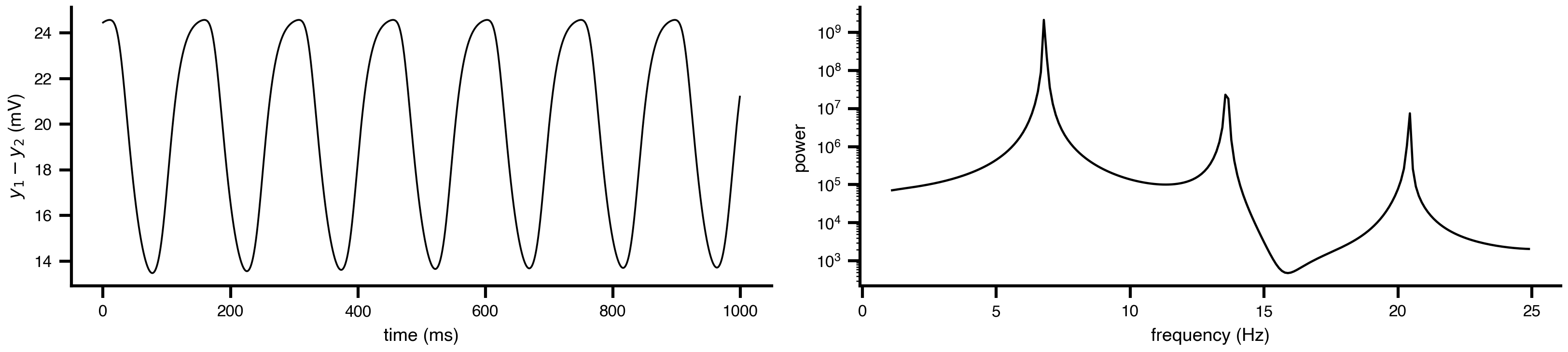
Figure 1: One column at its default drive. A clean limit cycle, and therefore a single sharp spectral line.

Stage 3 — drive it with noise

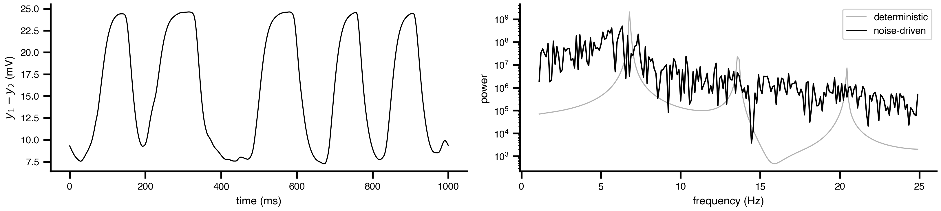
A deterministic column settles onto that limit cycle and stays there. Real cortex does not: Jansen and Rit drove the pyramidal population with a fluctuating input, and the broadened peak that produces is what makes the trace look like an EEG.

targets: puts the noise on one state variable rather than all six. y4 is the pyramidal population’s derivative state, which is where an afferent input enters.

Documented by Noise & stochastic integration.

STAGE3 = grow(
    STAGE2,
    "integration: {method: Heun, step_size: 0.5, duration: 9000.0, transient_time: 1000.0}",
    """integration:
  method: Heun
  step_size: 0.5
  duration: 9000.0
  transient_time: 1000.0
  noise:
    noise_type: gaussian
    targets: [y4]
    parameters: {sigma: {value: 0.002}}""",
)

driven = SimulationExperiment.from_string(STAGE3).run()
eeg_driven = np.asarray(driven.observations.eeg.data).squeeze()
print(f"rhythm at {peak_hz(eeg_driven):.2f} Hz, amplitude sd {eeg_driven.std():.2f} mV")

INFO [tvbo.run] [+0s] STEP 1: Running simulation...
INFO [tvbo.run] [+1s]   Simulation period: 9000.0 ms, dt: 0.5 ms
INFO [tvbo.run] [+1s]   Transient period: 1000.0 ms (settled on (-1000.0, 0], warm-started via update_history)
INFO [tvbo.run] [+1s]   Simulation complete.
INFO [tvbo.run] [+1s] Experiment complete.

rhythm at 6.33 Hz, amplitude sd 6.21 mV

Code

f2, p2 = spectrum(eeg_driven)
b2 = (f2 > 1) & (f2 < 25)

fig, axes = plt.subplots(1, 2, figsize=(11, 2.6))
axes[0].plot(np.arange(2000) * DT, eeg_driven[:2000], lw=0.9)
axes[0].set_xlabel("time (ms)"); axes[0].set_ylabel("$y_1 - y_2$ (mV)")
axes[1].semilogy(freqs[band], power[band], lw=0.9, color="0.7", label="deterministic")
axes[1].semilogy(f2[b2], p2[b2], lw=1.1, label="noise-driven")
axes[1].set_xlabel("frequency (Hz)"); axes[1].set_ylabel("power"); axes[1].legend(fontsize=8)
plt.tight_layout(); plt.show()

Figure 2: The same column driven by noise. The line broadens into a band, and the amplitude fluctuates from cycle to cycle.

Stage 4 — sweep the drive

One run answers nothing about how the drive sets the rhythm. An explorations block turns the single experiment into a grid over the physiological input range, and record: says which observation to keep per cell so the result stays small.

Documented by Parameter exploration.

DRIVES = [0.12, 0.17, 0.22, 0.27, 0.32]

STAGE4 = STAGE3 + f"""
explorations:
  drive:
    label: "Mean input to the pyramidal population"
    mode: product
    record: [eeg]
    space:
      mu:
        explored_values: {DRIVES}
"""

swept = SimulationExperiment.from_string(STAGE4).run()
cells = np.asarray(swept.explorations.drive.observations["eeg"])
column_hz = [peak_hz(cells[i]) for i in range(cells.shape[0])]
print({mu: round(hz, 2) for mu, hz in zip(DRIVES, column_hz)})

INFO [tvbo.run] [+0s] STEP 1: Running simulation...
INFO [tvbo.run] [+1s]   Simulation period: 9000.0 ms, dt: 0.5 ms
INFO [tvbo.run] [+1s]   Transient period: 1000.0 ms (settled on (-1000.0, 0], warm-started via update_history)
INFO [tvbo.run] [+1s]   Simulation complete.
INFO [tvbo.run] [+1s] STEP 2: Running explorations...
INFO [tvbo.run] [+1s]   > drive
INFO [tvbo.run]   grid batch 1/1 (100%)
INFO [tvbo.run] [+1s]   Explorations complete.
INFO [tvbo.run] [+1s] Experiment complete.

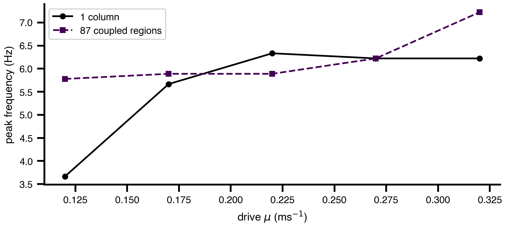
{0.12: 3.67, 0.17: 5.67, 0.22: 6.33, 0.27: 6.22, 0.32: 6.22}

The column’s rhythm rides on its drive, which is Jansen and Rit’s own result: the same circuit sits in the theta band when weakly driven and climbs toward alpha as the input grows.

Stage 5 — put it on a connectome

Replace the one node with a real network and say how activity travels between nodes. Two things change: network gains an iri and a weight transform, and a coupling entry names the model’s own input port.

The coupling key is not a name you invent. Dynamics.from_db("JansenRit").coupling_inputs names it c_glob, and it enters the pyramidal equation exactly where mu does.

Documented by Network specification and Coupling functions.

STAGE5 = grow(
    STAGE4,
    "network:\n  number_of_nodes: 1",
    """network:
  iri: tvbo:DesikanKilliany
  transforms:
    - name: weight
      equation: {rhs: "weight / mean(weight[weight > 0])"}
  coupling:
    c_glob:
      iri: tvbo:SigmoidalJansenRit
      parameters: {a: {value: 25.0}}""",
)

network = SimulationExperiment.from_string(STAGE5).run()
net_cells = np.asarray(network.explorations.drive.observations["eeg"])
network_hz = [peak_hz(net_cells[i]) for i in range(net_cells.shape[0])]
print({mu: round(hz, 2) for mu, hz in zip(DRIVES, network_hz)})

INFO [tvbo.run] [+0s] STEP 1: Running simulation...
INFO [tvbo.run] [+2s]   Simulation period: 9000.0 ms, dt: 0.5 ms
INFO [tvbo.run] [+2s]   Transient period: 1000.0 ms (settled on (-1000.0, 0], warm-started via update_history)
INFO [tvbo.run] [+3s]   Simulation complete.
INFO [tvbo.run] [+3s] STEP 2: Running explorations...
INFO [tvbo.run] [+3s]   > drive
INFO [tvbo.run]   grid batch 1/5 (20%)
INFO [tvbo.run]   grid batch 2/5 (40%)
INFO [tvbo.run]   grid batch 3/5 (60%)
INFO [tvbo.run]   grid batch 4/5 (80%)
INFO [tvbo.run]   grid batch 5/5 (100%)
INFO [tvbo.run] [+5s]   Explorations complete.
INFO [tvbo.run] [+5s] Experiment complete.

{0.12: 5.78, 0.17: 5.89, 0.22: 5.89, 0.27: 6.22, 0.32: 7.22}

Code

fig, ax = plt.subplots(figsize=(6, 2.8))
ax.plot(DRIVES, column_hz, "o-", lw=1.4, label="1 column")
ax.plot(DRIVES, network_hz, "s--", lw=1.4, label="87 coupled regions")
ax.set_xlabel(r"drive $\mu$ (ms$^{-1}$)"); ax.set_ylabel("peak frequency (Hz)")
ax.legend(fontsize=8)
plt.tight_layout(); plt.show()

Figure 3: The same drive sweep, run on one column and on 87 coupled regions. Coupling supplies input the column cannot tell apart from its own drive, so the network’s rhythm stops tracking `mu`.

Two things that bite newcomers here

Normalize the connectome. The Desikan-Killiany matrix holds streamline counts in the hundreds of thousands. Fed in raw they swamp every intrinsic term. The transforms block rescales so the mean non-zero weight is \(1\), which puts the coupling gain on a scale you can reason about.

Jansen-Rit needs a saturating coupling function. tvbo:SigmoidalJansenRit bounds each edge’s contribution. Substituting tvbo:Linear on y1 makes the drive unbounded, and above a gain of roughly \(0.02\) on max-normalized weights the run diverges to inf rather than converging on anything.

Stage 6 — make it a study

A paper is not one experiment. A SimulationStudy holds several, shares blocks between them with YAML anchors, and declares the analyses and figures that turn results into the thing you publish.

Documented by Linked experiments in a SimulationStudy, Analyses, Specify a figure and Writing TVB-O YAML.

key: DriveAndCoupling
title: "Coupling competes with drive in setting the Jansen-Rit rhythm"

experiments:
  - id: 1
    label: "Single column, drive sweep"
    <<: *column_sweep
  - id: 2
    label: "Connectome, same drive sweep"
    <<: *network_sweep

analyses:
  peak_frequency:
    code_source: {module: rhythm, callable: peak_frequency}
    used:
      - {experiment: 1, output: observation__eeg}
      - {experiment: 2, output: observation__eeg}

figures:
  - name: fig1
    panels:
      a: {kind: line, layers: [{used: {analysis: peak_frequency}}]}

Where each block is documented

Stage	Block it adds	Page that owns it
1	`dynamics`, `network`, `integration`	The SimulationExperiment
2	`observations`	Observation models, Output specification
3	`integration.noise`	Noise & stochastic integration
4	`explorations`, `record`	Parameter exploration
5	`network.iri`, `transforms`, `coupling`	Network specification, Coupling functions
6	`experiments`, `analyses`, `figures`	SimulationStudy, Analyses, Figures

The blocks this thread never needed slot in the same way and are documented the same way: events and stimulation, fan-out over subjects, calling your own code, algorithms and loss functions.