* Owlready2 * Warning: ignoring cyclic subclass of/subproperty of, involving:
  http://uri.interlex.org/tgbugs/uris/readable/atlas/Space

INFO [tvbo.run] [+0s] STEP 1: Running simulation...
INFO [tvbo.run] [+1s]   Simulation period: 300000.0 ms, dt: 4.0 ms
INFO [tvbo.run] [+1s]   Transient period: 300000.0 ms (settled on (-300000.0, 0], warm-started via update_history)
INFO [tvbo.run] [+2s]   Simulation complete.
INFO [tvbo.run] [+2s] STEP 3: Running algorithms...
INFO [tvbo.run] [+2s]   Algorithms to run (dependency order): ['fic', 'fic_eib']
INFO [tvbo.run] [+2s] \n>>> Running algorithm: fic (seed=0)
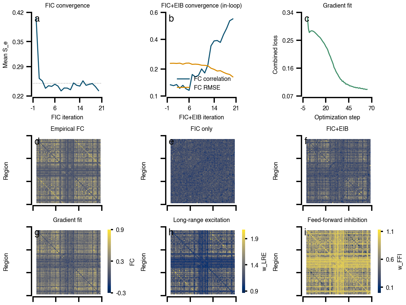
INFO [tvbo.run] Running fic algorithm for 200 iterations...
INFO [tvbo.run]   10/200: mean_S_e=0.2619, mean_S_i=0.0917, bold=0.9267
INFO [tvbo.run]   20/200: mean_S_e=0.2558, mean_S_i=0.0899, bold=0.8406
INFO [tvbo.run]   30/200: mean_S_e=0.2382, mean_S_i=0.0838, bold=0.7852
INFO [tvbo.run]   40/200: mean_S_e=0.2443, mean_S_i=0.0858, bold=0.7950
INFO [tvbo.run]   50/200: mean_S_e=0.2428, mean_S_i=0.0857, bold=0.7979
INFO [tvbo.run]   60/200: mean_S_e=0.2480, mean_S_i=0.0852, bold=0.8291
INFO [tvbo.run]   70/200: mean_S_e=0.2435, mean_S_i=0.0864, bold=0.8194
INFO [tvbo.run]   80/200: mean_S_e=0.2319, mean_S_i=0.0815, bold=0.7885
INFO [tvbo.run]   90/200: mean_S_e=0.2389, mean_S_i=0.0835, bold=0.7648
INFO [tvbo.run]   100/200: mean_S_e=0.2386, mean_S_i=0.0828, bold=0.7686
INFO [tvbo.run]   110/200: mean_S_e=0.2347, mean_S_i=0.0832, bold=0.8120
INFO [tvbo.run]   120/200: mean_S_e=0.2510, mean_S_i=0.0868, bold=0.8310
INFO [tvbo.run]   130/200: mean_S_e=0.2454, mean_S_i=0.0846, bold=0.8103
INFO [tvbo.run]   140/200: mean_S_e=0.2435, mean_S_i=0.0849, bold=0.8001
INFO [tvbo.run]   150/200: mean_S_e=0.2561, mean_S_i=0.0872, bold=0.8289
INFO [tvbo.run]   160/200: mean_S_e=0.2453, mean_S_i=0.0844, bold=0.8316
INFO [tvbo.run]   170/200: mean_S_e=0.2477, mean_S_i=0.0865, bold=0.7771
INFO [tvbo.run]   180/200: mean_S_e=0.2494, mean_S_i=0.0867, bold=0.8349
INFO [tvbo.run]   190/200: mean_S_e=0.2421, mean_S_i=0.0849, bold=0.7866
INFO [tvbo.run]   200/200: mean_S_e=0.2325, mean_S_i=0.0821, bold=0.7934
INFO [tvbo.run] fic complete! (tuning 3.6s, 200 iters; post-tuning eval 2.5s)
INFO [tvbo.run] [+8s]   fic done: 6.3s wall (tuning + post-tuning eval)
INFO [tvbo.run] [+8s] \n>>> Running algorithm: fic_eib (seed=0)
INFO [tvbo.run] [+8s]     (using state from dependency: fic)
INFO [tvbo.run]   Using passed bold buffer (200 samples, using last 150)
INFO [tvbo.run] Running fic_eib algorithm for 2000 iterations...
INFO [tvbo.run]   100/2000: fc_corr=0.1287, fc_rmse=0.2789, mean_S_e=0.2413, mean_S_i=0.0833, bold=0.7799, fc_inloop=0.0193
INFO [tvbo.run]   200/2000: fc_corr=0.1362, fc_rmse=0.2777, mean_S_e=0.2387, mean_S_i=0.0838, bold=0.8183, fc_inloop=0.0197
INFO [tvbo.run]   300/2000: fc_corr=0.1110, fc_rmse=0.2797, mean_S_e=0.2618, mean_S_i=0.0891, bold=0.8732, fc_inloop=0.0199
INFO [tvbo.run]   400/2000: fc_corr=0.1307, fc_rmse=0.2727, mean_S_e=0.2555, mean_S_i=0.0866, bold=0.8541, fc_inloop=0.0270
INFO [tvbo.run]   500/2000: fc_corr=0.1078, fc_rmse=0.2795, mean_S_e=0.2561, mean_S_i=0.0882, bold=0.8374, fc_inloop=0.0207
INFO [tvbo.run]   600/2000: fc_corr=0.0972, fc_rmse=0.2801, mean_S_e=0.2585, mean_S_i=0.0875, bold=0.8604, fc_inloop=0.0215
INFO [tvbo.run]   700/2000: fc_corr=0.2036, fc_rmse=0.2716, mean_S_e=0.2686, mean_S_i=0.0889, bold=0.8819, fc_inloop=0.0264
INFO [tvbo.run]   800/2000: fc_corr=0.1872, fc_rmse=0.2729, mean_S_e=0.2499, mean_S_i=0.0834, bold=0.8246, fc_inloop=0.0244
INFO [tvbo.run]   900/2000: fc_corr=0.1980, fc_rmse=0.2713, mean_S_e=0.2520, mean_S_i=0.0843, bold=0.8540, fc_inloop=0.0248
INFO [tvbo.run]   1000/2000: fc_corr=0.2409, fc_rmse=0.2656, mean_S_e=0.2560, mean_S_i=0.0853, bold=0.8273, fc_inloop=0.0295
INFO [tvbo.run]   1100/2000: fc_corr=0.2136, fc_rmse=0.2649, mean_S_e=0.2755, mean_S_i=0.0885, bold=0.9312, fc_inloop=0.0329
INFO [tvbo.run]   1200/2000: fc_corr=0.2672, fc_rmse=0.2620, mean_S_e=0.2593, mean_S_i=0.0823, bold=0.8516, fc_inloop=0.0337
INFO [tvbo.run]   1300/2000: fc_corr=0.3958, fc_rmse=0.2457, mean_S_e=0.2601, mean_S_i=0.0824, bold=0.8625, fc_inloop=0.0458
INFO [tvbo.run]   1400/2000: fc_corr=0.4288, fc_rmse=0.2379, mean_S_e=0.2934, mean_S_i=0.0902, bold=0.9899, fc_inloop=0.0519
INFO [tvbo.run]   1500/2000: fc_corr=0.4316, fc_rmse=0.2269, mean_S_e=0.2685, mean_S_i=0.0840, bold=0.8742, fc_inloop=0.0658
INFO [tvbo.run]   1600/2000: fc_corr=0.4189, fc_rmse=0.2291, mean_S_e=0.2791, mean_S_i=0.0864, bold=0.9369, fc_inloop=0.0655
INFO [tvbo.run]   1700/2000: fc_corr=0.4708, fc_rmse=0.2181, mean_S_e=0.2745, mean_S_i=0.0841, bold=0.9435, fc_inloop=0.0766
INFO [tvbo.run]   1800/2000: fc_corr=0.5127, fc_rmse=0.2090, mean_S_e=0.2616, mean_S_i=0.0802, bold=0.8000, fc_inloop=0.0846
INFO [tvbo.run]   1900/2000: fc_corr=0.5642, fc_rmse=0.2036, mean_S_e=0.2507, mean_S_i=0.0773, bold=0.8106, fc_inloop=0.0880
INFO [tvbo.run]   2000/2000: fc_corr=0.5766, fc_rmse=0.1875, mean_S_e=0.2381, mean_S_i=0.0720, bold=0.6987, fc_inloop=0.1087
INFO [tvbo.run] fic_eib complete! (tuning 29.5s, 2000 iters; post-tuning eval 1.4s)
INFO [tvbo.run] [+39s]   fic_eib done: 31.0s wall (tuning + post-tuning eval)
INFO [tvbo.run] [+39s]   Algorithms complete. Results: ['fic', 'fic_eib']
INFO [tvbo.run] [+39s] STEP 4: Running optimization...
INFO [tvbo.run] [+39s]   Preparing optimization model (t1=300000.0ms, dt=4.0ms, solver=Heun)
INFO [tvbo.run]   step 0/66: loss=0.322559
INFO [tvbo.run]   step 1/66: loss=0.287416
INFO [tvbo.run]   step 2/66: loss=0.274887
INFO [tvbo.run]   step 3/66: loss=0.278554
INFO [tvbo.run]   step 4/66: loss=0.280383
INFO [tvbo.run]   step 5/66: loss=0.280416
INFO [tvbo.run]   step 6/66: loss=0.279506
INFO [tvbo.run]   step 7/66: loss=0.277855
INFO [tvbo.run]   step 8/66: loss=0.275488
INFO [tvbo.run]   step 9/66: loss=0.272472
INFO [tvbo.run]   step 10/66: loss=0.269536
INFO [tvbo.run]   step 11/66: loss=0.266342
INFO [tvbo.run]   step 12/66: loss=0.263162
INFO [tvbo.run]   step 13/66: loss=0.260752
INFO [tvbo.run]   step 14/66: loss=0.257829
INFO [tvbo.run]   step 15/66: loss=0.25353
INFO [tvbo.run]   step 16/66: loss=0.248843
INFO [tvbo.run]   step 17/66: loss=0.244591
INFO [tvbo.run]   step 18/66: loss=0.240711
INFO [tvbo.run]   step 19/66: loss=0.235674
INFO [tvbo.run]   step 20/66: loss=0.229598
INFO [tvbo.run]   step 21/66: loss=0.225132
INFO [tvbo.run]   step 22/66: loss=0.219524
INFO [tvbo.run]   step 23/66: loss=0.21077
INFO [tvbo.run]   step 24/66: loss=0.202817
INFO [tvbo.run]   step 25/66: loss=0.196753
INFO [tvbo.run]   step 26/66: loss=0.18802
INFO [tvbo.run]   step 27/66: loss=0.180813
INFO [tvbo.run]   step 28/66: loss=0.172838
INFO [tvbo.run]   step 29/66: loss=0.161963
INFO [tvbo.run]   step 30/66: loss=0.156707
INFO [tvbo.run]   step 31/66: loss=0.149464
INFO [tvbo.run]   step 32/66: loss=0.143933
INFO [tvbo.run]   step 33/66: loss=0.139504
INFO [tvbo.run]   step 34/66: loss=0.133502
INFO [tvbo.run]   step 35/66: loss=0.129095
INFO [tvbo.run]   step 36/66: loss=0.123936
INFO [tvbo.run]   step 37/66: loss=0.121912
INFO [tvbo.run]   step 38/66: loss=0.116935
INFO [tvbo.run]   step 39/66: loss=0.117669
INFO [tvbo.run]   step 40/66: loss=0.112658
INFO [tvbo.run]   step 41/66: loss=0.112126
INFO [tvbo.run]   step 42/66: loss=0.107734
INFO [tvbo.run]   step 43/66: loss=0.108419
INFO [tvbo.run]   step 44/66: loss=0.106081
INFO [tvbo.run]   step 45/66: loss=0.105278
INFO [tvbo.run]   step 46/66: loss=0.102378
INFO [tvbo.run]   step 47/66: loss=0.102327
INFO [tvbo.run]   step 48/66: loss=0.101048
INFO [tvbo.run]   step 49/66: loss=0.100245
INFO [tvbo.run]   step 50/66: loss=0.0991085
INFO [tvbo.run]   step 51/66: loss=0.0976807
INFO [tvbo.run]   step 52/66: loss=0.097972
INFO [tvbo.run]   step 53/66: loss=0.096102
INFO [tvbo.run]   step 54/66: loss=0.0970327
INFO [tvbo.run]   step 55/66: loss=0.0957913
INFO [tvbo.run]   step 56/66: loss=0.0947468
INFO [tvbo.run]   step 57/66: loss=0.0961339
INFO [tvbo.run]   step 58/66: loss=0.0940019
INFO [tvbo.run]   step 59/66: loss=0.0936006
INFO [tvbo.run]   step 60/66: loss=0.0940143
INFO [tvbo.run]   step 61/66: loss=0.0920273
INFO [tvbo.run]   step 62/66: loss=0.0924769
INFO [tvbo.run]   step 63/66: loss=0.091674
INFO [tvbo.run]   step 64/66: loss=0.090727
INFO [tvbo.run]   step 65/66: loss=0.0910322
INFO [tvbo.run] [+256s]   Optimization complete.
INFO [tvbo.run] [+256s] Experiment complete.
INFO [tvbo.cli] done: ExperimentResult
INFO [tvbo.cli] wrote ['/Users/leonmartin_bih/tools/tvbo/docs/_build/EI_Tuning_tvboptim/derivatives/tvbo/exp-3_model-ReducedWongWangEIB_result.h5', '/Users/leonmartin_bih/tools/tvbo/docs/_build/EI_Tuning_tvboptim/derivatives/tvbo/exp-3_model-ReducedWongWangEIB_result.yaml']
INFO [tvbo.cli] rendering 1 figure(s) -> /Users/leonmartin_bih/tools/tvbo/docs/_build/EI_Tuning_tvboptim/docs/figures
INFO [tvbo.cli] ei_tuning FAILED (KeyError: '{}')
WARNING [tvbo.cli] figure rendering failed (RuntimeError: 1 of 1 figures did not render:
  ei_tuning: KeyError: '{}'); the experiment results are saved. Re-run `tvbo figure render /Users/leonmartin_bih/tools/tvbo/docs/examples/fitting/EI_Tuning_tvboptim.yaml` to retry.