Most simulations need something to happen: a stimulation pulse, a task input, a perturbation to probe the model’s response. In TVBO these are events, and the most common kind is a stimulus: a time-dependent signal injected into the model.
A stimulus is not a hardcoded array of numbers. It is a symbolic equation in time, which is what lets the same object serialize to YAML, render to every backend, and stay reproducible alongside the model.
Anatomy of a stimulus
An event answers three questions:
Question
Field
Example
Into what?
the event’s name
I, the model port it drives
What shape?
equation.rhs + parameters
a rectangular pulse in t
Where?
nodes / weights
which regions, how strongly
A rectangular pulse of amplitude \(A\), onset \(t_0\) and width \(w\) is
\[
s(t) \;=\;
\begin{cases}
A, & t_0 \le t < t_0 + w \\[2pt]
0, & \text{otherwise}
\end{cases}
\]
written with SymPy’s Piecewise:
events:I: # <- the model port being drivenevent_type: stimulusequation:rhs:"Piecewise((amplitude, (t >= onset) & (t < onset + width)), (0.0, True))"parameters:amplitude:{value:5.0}onset:{value:100.0,unit: ms}width:{value:50.0,unit: ms}
Any expression in t and the event’s own parameters is valid: a Gaussian, a ramp or a sinusoid all work the same way.
The event name is the model port, not a label
The name binds the signal to a symbol in the model’s equations. Generic2dOscillator has
\[\dot V = d\,\tau\left(I\gamma - V^3 f + V^2 e + \ldots\right)\]
so naming the event I injects the signal into that input term. Naming it something descriptive like stimulus binds to nothing and is silently ignored: no error, no warning, just an unchanged simulation.
Worse, naming it after a state variable (V) overwrites that state inside the derivative function rather than driving an input. The run “responds”, but the trajectory is unphysical. Check the model’s equations and pick an input symbol.
* Owlready2 * Warning: ignoring cyclic subclass of/subproperty of, involving:
  http://uri.interlex.org/tgbugs/uris/readable/atlas/Space

INFO [tvbo.run] [+0s] STEP 1: Running simulation...
INFO [tvbo.run] [+0s]   Simulation period: 300.0 ms, dt: 0.05 ms
INFO [tvbo.run] [+0s]   Simulation complete.
INFO [tvbo.run] [+0s] Experiment complete.
INFO [tvbo.run] [+0s] STEP 1: Running simulation...
INFO [tvbo.run] [+0s]   Simulation period: 300.0 ms, dt: 0.05 ms
INFO [tvbo.run] [+0s]   Simulation complete.
INFO [tvbo.run] [+0s] Experiment complete.
INFO [tvbo.run] [+0s] STEP 1: Running simulation...
INFO [tvbo.run] [+0s]   Simulation period: 300.0 ms, dt: 0.05 ms
INFO [tvbo.run] [+0s]   Simulation complete.
INFO [tvbo.run] [+0s] Experiment complete.
Code
fig, ax = plt.subplots(figsize=(9, 3.2))ax.axvspan(100, 150, color="0.85", zorder=0, label="pulse")ax.plot(t, baseline, lw=1.0, label="baseline (no stimulus)")for amp, V in runs.items(): ax.plot(t, V, lw=1.2, label=f"amplitude = {amp}")ax.set_xlabel("time (ms)")ax.set_ylabel("V")ax.legend(fontsize=8, loc="upper left")plt.tight_layout()plt.show()
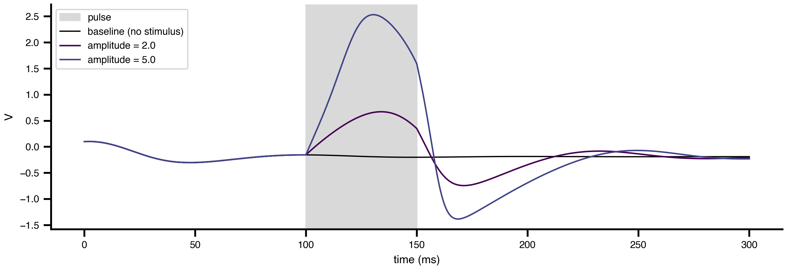
Figure 1: A 50 ms pulse into the model’s input port. The shaded band marks the stimulation window; stronger drive produces a larger excursion, and the model returns to baseline afterwards.
Response inside the stimulation window
import pandas as pddef window(V, lo=100, hi=150): seg = V[(t > lo) & (t < hi)]returnround(float(seg.max() - seg.min()), 3), round(float(seg.mean()), 3)rows = []for name, V in [("baseline", baseline)] + [(f"amplitude {a}", v) for a, v in runs.items()]: rng, mean = window(V) rows.append({"run": name, "range during window": rng, "mean V during window": mean})pd.DataFrame(rows)
Table 1
run
range during window
mean V during window
0
baseline
0.046
-0.181
1
amplitude 2.0
0.824
0.429
2
amplitude 5.0
2.682
1.709
The response scales with amplitude and the model returns to its baseline oscillation once the pulse ends, the signature of a stimulus entering through an input term rather than overwriting the state.
Targeting regions
On a network, nodes and weights decide where the signal lands:
events:I:event_type: stimulusequation:rhs:"Piecewise((amplitude, (t >= onset) & (t < onset + width)), (0.0, True))"parameters:amplitude:{value:5.0}onset:{value:100.0}width:{value:50.0}nodes:[0,12,34] # which regions receive itweights:[1.0,0.5,0.5] # how strongly each one does
Omitting nodes applies the stimulus to every region equally. This is how a focal perturbation is expressed declaratively, whether that is a single stimulated region or an electrode’s projection profile.
The other event types
stimulus is one of four mechanisms in the schema. The others trigger on a condition rather than supplying a continuous signal:
event_type
Triggers when
Status on the JAX/tvboptim backend
stimulus / stimulation
always, a continuous signal in t
working (shown above)
continuous
a condition expression crosses zero
working
discrete
a condition evaluates true at a step
working, but see caveat: it is currently an alias for continuous
preset_time
at listed trigger_times
not emitted; see caveat
A condition-triggered event is declared like a stimulus, plus the condition that arms it and the waveform it then emits as a function of tau, the time since it fired:
events:burst:event_type: continuouscondition:{rhs:"x - 0.05"} # arms on the upward zero crossingcondition_states:[x] # the states the condition readsaffect:{rhs:"q * (tau/w) * exp(-tau/w)"}parameters:q:{value:5.0}w:{value:80.0,unit: ms}target_variable: x # the port it drives, as for a stimulustarget_regions:[ctx-lh-superiortemporal, ctx-rh-superiortemporal]
target_variable matters here for exactly the reason it does for a stimulus: the event reaches the derivative through a port, and one that binds to nothing is computed each step and discarded. Each node arms independently on its own crossing, and triggering is detected by a per-step sign change, so the onset resolves to the integration step rather than to a polished root.
Two gaps remain
discrete is accepted and produces output byte-identical to continuous: both route through the same zero-crossing branch, so the “evaluates true at a step” semantics in the table above are not yet distinct.
A preset_time event runs without error but produces output byte-identical to the unstimulated baseline, because the code generator emits no branch for it and it is therefore silently inert.
Threshold-and-reset dynamics (spiking, refractory periods) with per-step semantics are still best expressed through models that build the reset into their own equations, or through the NeuroML route, which has explicit event semantics.