Coupling Functions

How activity in one region becomes input to another

2Specify·Networks & connectomes

Part of the running example, where stage 5 adds a connectome and a coupling function.

A network model is not just nodes and a connectome. It also needs a rule that turns the state of one region into the input another region receives. That rule is the coupling function, and it matters as much as the node dynamics: the same neural mass model on the same connectome produces different brain-wide behaviour depending on how regions talk to each other.

The two-stage formalism

TVBO splits coupling into two expressions, applied in sequence.

Stage 1 — pre-synaptic, per edge. For every connection \(j \to i\) a pre_expression is evaluated, then weighted by the structural connectivity \(W_{ij}\) and summed over all sources:

\[ g_i \;=\; \sum_{j} W_{ij}\;\mathrm{pre}\!\left(x_i,\; x_j(t - \tau_{ij})\right) \]

Stage 2 — post-synaptic, per node. The aggregated signal \(g_i\) (written gx in the YAML) passes through a post_expression to give the value injected into the node’s equations:

\[ c_i \;=\; \mathrm{post}\!\left(g_i\right) \]

Two symbols carry the meaning:

Symbol	In YAML	Meaning
\(x_j\)	x_j	state of the source (remote) region, delayed by \(\tau_{ij}\)
\(x_i\)	x_i	state of the target (local) region, not delayed
\(g_i\)	gx	weighted sum over incoming edges, available to post_expression

The split is what makes the formalism efficient: anything that depends only on the sum belongs in post_expression and is evaluated once per node, not once per edge.

The delay \(\tau_{ij} = L_{ij}/v\) comes from tract length and conduction speed. Set delayed: false for an instantaneous approximation.

The curated library

import pandas as pd
from tvbo import Coupling

rows = []
for name in Coupling.list_db():
    c = Coupling.from_db(name)
    rows.append({
        "Coupling": name,
        "pre(x_i, x_j)": c.pre_expression.rhs,
        "post(gx)": c.post_expression.rhs,
        "delayed": c.delayed,
    })
pd.DataFrame(rows)

Table 1

	Coupling	pre(x_i, x_j)	post(gx)	delayed
0	Difference	-x_i + x_j	a*gx	True
1	FastLinearCoupling	local_states	G * gx + b	False
2	HyperbolicTangent	a*(tanh((b*x_j - midpoint)/sigma) + 1)	gx	True
3	KuramotoCoupling	sin(-x_i + x_j)	a*gx/N	True
4	Linear	x_j	a*gx + b	True
5	PreSigmoidal	H*(Q + tanh(G*(P*x_j - theta)))	gx	True
6	Scaling	x_j	a*gx	True
7	Sigmoidal	x_j	cmin + (cmax - cmin)/(exp((-a)*(gx - midpoint)...	True
8	SigmoidalJansenRit	cmin + (cmax - cmin)/(exp(r*(midpoint - (x_j[0...	a*gx	True

Read the table structurally rather than by name:

• pre = x_j: the node simply receives its neighbours’ activity. Linear, Sigmoidal, Scaling.
• pre contains x_i: the input depends on the difference between the two regions, so the coupling is diffusive and vanishes when regions agree. Difference, Kuramoto.
• non-linear post: the summed input saturates. Sigmoidal, HyperbolicTangent.

What the transfer functions look like

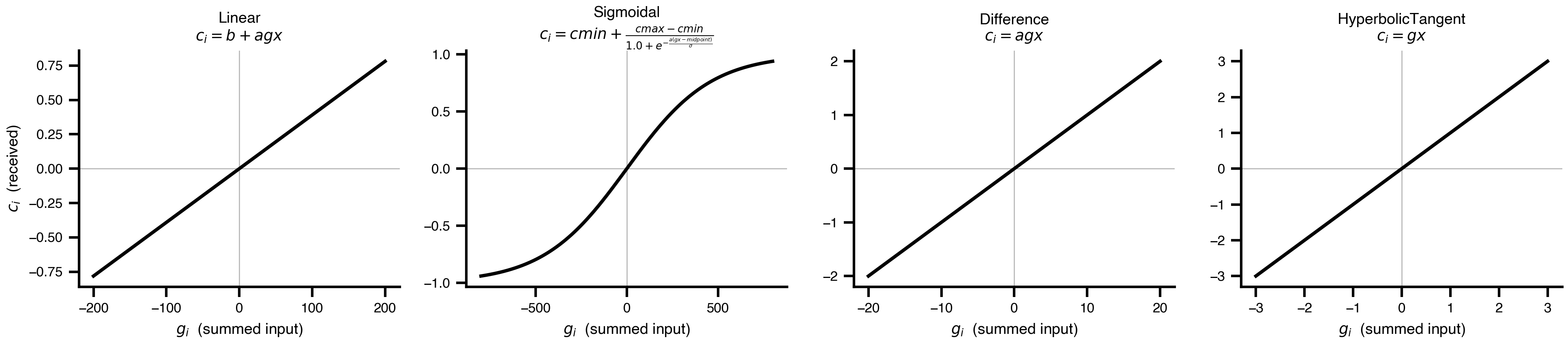
The post_expression is where a coupling’s character shows. Below, each curve is the node’s received input \(c_i\) as a function of the aggregated signal \(g_i\), using each coupling’s default parameters.

import numpy as np
import sympy as sp
import matplotlib.pyplot as plt
import bsplot

bsplot.style.use("tvbo")

# Defaults put these on very different scales, so sweep each over a range
# where its shape is actually visible.
SHOW = {"Linear": 200.0, "Sigmoidal": 800.0, "Difference": 20.0, "HyperbolicTangent": 3.0}
gx = sp.Symbol("gx")

fig, axes = plt.subplots(1, 4, figsize=(13, 3.0))
for ax, (name, span) in zip(axes, SHOW.items()):
    c = Coupling.from_db(name)
    subs = {sp.Symbol(k): v.value for k, v in c.parameters.items()}
    expr = sp.sympify(c.post_expression.rhs).subs(subs)
    f = sp.lambdify(gx, expr, "numpy")

    xs = np.linspace(-span, span, 400)
    ys = np.broadcast_to(np.asarray(f(xs), dtype=float), xs.shape)

    ax.plot(xs, ys, lw=2)
    ax.axhline(0, color="0.7", lw=0.6, zorder=0)
    ax.axvline(0, color="0.7", lw=0.6, zorder=0)
    ax.set_title(f"{name}\n$c_i = {sp.latex(sp.sympify(c.post_expression.rhs))}$", fontsize=9)
    ax.set_xlabel("$g_i$  (summed input)")
axes[0].set_ylabel("$c_i$  (received)")
plt.tight_layout()
plt.show()

Figure 1: Post-synaptic transfer functions. The x-ranges differ deliberately: each coupling’s default parameters set its own natural scale.

Linear and Difference scale their input without bound. Sigmoidal and HyperbolicTangent saturate, so a strongly-driven region cannot receive arbitrarily large input — often the difference between a model that settles and one that diverges.

Using a coupling in an experiment

Reference a curated coupling by its ontology iri. The key must be the coupling input declared by the model — for models ported from TVB that is c_glob:

from tvbo import SimulationExperiment

LINEAR = """
label: "Linear coupling on the DK connectome"
dynamics:
  iri: tvbo:Generic2dOscillator
network:
  iri: tvbo:DesikanKilliany
  transforms:
    - name: weight
      equation: {rhs: "weight / mean(weight[weight > 0])"}   # mean non-zero weight -> 1
  coupling:
    c_glob:
      iri: tvbo:Linear
      delayed: false
      incoming_states: [V]
integration:
  method: Heun
  step_size: 0.1
  duration: 600.0
  transient_time: 200.0
"""
exp = SimulationExperiment.from_string(LINEAR)
print(exp.dynamics.name, "on", exp.network.number_of_nodes, "regions")
print("accepted coupling inputs:", list(exp.dynamics.coupling_inputs))

* Owlready2 * Warning: ignoring cyclic subclass of/subproperty of, involving:
  http://uri.interlex.org/tgbugs/uris/readable/atlas/Space

Generic2dOscillator on 87 regions
accepted coupling inputs: ['c_glob', 'local_coupling']

Two fields decide how the coupling binds to the model:

• incoming_states: [V]: which state variable of the source region plays the role of \(x_j\).
• delayed: whether \(x_j\) is read from the delayed history buffer.

The key is the coupling input, not a name you choose

A model declares which coupling inputs it accepts, as printed above. Keying the block anything else leaves the model’s input unsatisfied and the run fails with PRE_USES_LOCAL is True but no local_states were configured.

Normalize the connectome, and mind the step size

Structural connectomes are stored in their native units — the dTOR Desikan-Killiany matrix holds streamline counts with a maximum near \(4.6\times10^{5}\). Feeding those raw into any coupling makes the drive astronomically large and the simulation returns NaN immediately. The transforms block above rescales so the mean non-zero weight is \(1\), which keeps coupling strengths \(\mathcal{O}(1)\).

Step size matters too: this model on this connectome diverges at step_size: 0.5 with Heun and is stable at 0.1. If a network run returns NaN, suspect weight scale and step size before the coupling itself.

The effect on network dynamics

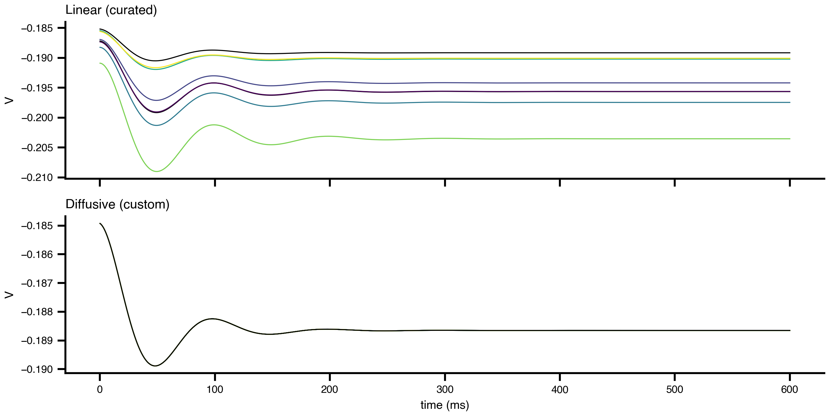
Coupling does not merely add input — it decides whether regions keep their own identity or collapse onto a common trajectory. Compare the curated Linear coupling with a diffusive one written by hand.

Because a diffusive pre_expression reads the local state \(x_i\), it must declare local_states as well:

\[ g_i = \sum_j W_{ij}\,\bigl(x_j - x_i\bigr), \qquad c_i = G \tanh\!\left(\frac{g_i}{n}\right) \]

DIFFUSIVE = """
label: "Custom saturating diffusive coupling"
dynamics:
  iri: tvbo:Generic2dOscillator
network:
  iri: tvbo:DesikanKilliany
  transforms:
    - name: weight
      equation: {rhs: "weight / mean(weight[weight > 0])"}
  coupling:
    c_glob:
      label: "Saturating diffusive coupling"
      delayed: false
      incoming_states: [V]
      local_states: [V]          # required: pre_expression uses x_i
      parameters:
        G: {value: 0.4}
        n: {value: 2.0}
      pre_expression: {rhs: "x_j - x_i"}
      post_expression: {rhs: "G*tanh(gx/n)"}
integration:
  method: Heun
  step_size: 0.1
  duration: 600.0
  transient_time: 200.0
"""

runs = {}
for name, spec in [("Linear (curated)", LINEAR), ("Diffusive (custom)", DIFFUSIVE)]:
    runs[name] = SimulationExperiment.from_string(spec).run().integration.data.sel(variable="V")

INFO [tvbo.run] [+0s] STEP 1: Running simulation...
INFO [tvbo.run] [+2s]   Simulation period: 600.0 ms, dt: 0.1 ms
INFO [tvbo.run] [+2s]   Transient period: 200.0 ms (settled on (-200.0, 0], warm-started via update_history)
INFO [tvbo.run] [+2s]   Simulation complete.
INFO [tvbo.run] [+2s] Experiment complete.
INFO [tvbo.run] [+0s] STEP 1: Running simulation...
INFO [tvbo.run] [+1s]   Simulation period: 600.0 ms, dt: 0.1 ms
INFO [tvbo.run] [+1s]   Transient period: 200.0 ms (settled on (-200.0, 0], warm-started via update_history)
INFO [tvbo.run] [+1s]   Simulation complete.
INFO [tvbo.run] [+1s] Experiment complete.

fig, axes = plt.subplots(2, 1, figsize=(9, 4.6), sharex=True)
for ax, (name, V) in zip(axes, runs.items()):
    ax.plot(V.time, V.isel(node=slice(0, 8)), lw=0.8)
    ax.set_ylabel("V")
    ax.set_title(name, loc="left", fontsize=10)
axes[-1].set_xlabel("time (ms)")
plt.tight_layout()
plt.show()

Figure 2: Eight regions under two couplings. Diffusive coupling collapses the regions onto one trajectory; the curated Linear coupling does not.

rows = []
for name, V in runs.items():
    arr = np.asarray(V)                                   # (time, node)
    rows.append({
        "Coupling": name,
        "mean |V|": round(float(np.abs(arr).mean()), 4),
        "across-region SD": round(float(arr.std(axis=1).mean()), 4),
    })
pd.DataFrame(rows)

Table 2

	Coupling	mean |V|	across-region SD
0	Linear (curated)	0.1927	0.0044
1	Diffusive (custom)	0.1886	0.0000

The across-region SD is the number to read: it measures how far apart the regions stay. The diffusive coupling drives it to zero — every region converges on the same trajectory, because the term \(\sum_j W_{ij}(x_j - x_i)\) vanishes only when \(x_i = x_j\). That is synchronization produced by the coupling rule alone, on an unchanged connectome and an unchanged node model.

Parameters declared in the block are substituted into both expressions, so G and n can be swept in an exploration or fitted in an optimization exactly like model parameters.

If pre uses x_i, declare local_states

incoming_states binds \(x_j\); local_states binds \(x_i\). Omitting local_states on a diffusive coupling fails with PRE_USES_LOCAL is True but no local_states were configured. Curated diffusive couplings such as Difference and Kuramoto already carry it, which is why referencing them by iri needs no extra field — you supply it only when writing the expression yourself.

Choosing one

If you want…	Use	Why
A neutral starting point	Linear	Input scales with neighbours’ activity; fewest assumptions
Bounded input, no divergence	Sigmoidal, HyperbolicTangent	Saturating post caps drive on strongly-connected regions
Regions to synchronize	Difference, Kuramoto	Diffusive: the term vanishes as \(x_i \to x_j\)
Phase models	Kuramoto	pre is \(\sin(x_j - x_i)\), the canonical phase interaction
A published model reproduced	the one that paper used	Coupling is part of the model, not a free choice

Related

• Networks & connectomes: the \(W_{ij}\) this all runs on.
• Heterogeneous edges: per-edge coupling instead of one rule.
• Coupling schema: every field.
• Bifurcation & stability: coupling strength is the classic bifurcation parameter for a network model.

Used in published replications

11 peer-reviewed studies whose TVB-O recipe writes what this page documents.

• Acoustic & Stimulation — How far back a network listens is set by its conduction delays
• Deco (2014) — How Local Excitation-Inhibition Ratio Impacts the Whole Brain Dynamics
• Deco (2018) — Whole-Brain Multimodal Neuroimaging Model Using Serotonin Receptor Maps Explains Non-linear Functional Effects of LSD
• Feedback & Inhibition — A tuning algorithm declared beside the model it tunes
• Herzog (2024) — Neural mass modeling for the masses: Democratizing access to whole-brain biophysical modeling with FastDMF
• Jansen (1995) — Electroencephalogram and visual evoked potential generation in a mathematical model of coupled cortical columns
• Koller (2024) — Human connectome topology directs cortical traveling waves and shapes frequency gradients
• Pang (2023) — Geometric constraints on human brain function
• Schirner (2023) — Learning how network structure shapes decision-making for bio-inspired computing
• Stefanovski (2019) — Linking Molecular Pathways and Large-Scale Computational Modeling to Assess Candidate Disease Mechanisms and Pharmacodynamics in Alzheimer's Disease
• Taher (2019) — Enhancing power grid synchronization and stability through time-delayed feedback control