import os

device_count = os.environ.get("TVBO_XLA_DEVICE_COUNT", "8")
os.environ["XLA_FLAGS"] = f"--xla_force_host_platform_device_count={device_count}"

import jax

jax.config.update("jax_enable_x64", True)

import jax.numpy as jnp
import numpy as np

from tvbo import SimulationExperiment

# Kuramoto oscillators on the Desikan-Killiany connectome; the exploration sweeps
# network.conduction_speed (a DenseLengthGraph `speed` leaf) from 0.5 to 6 mm/ms.
exp = SimulationExperiment.from_db("Delay_Speed_Synchronization")
results = exp.run("tvboptim", mode="exploration")

# Order parameter R vs conduction speed (labeled xarray keyed by the swept axis).
sweep = results.explorations.speed_sweep.as_grid()
speeds = np.asarray(sweep["network.conduction_speed"].values)
R = np.asarray(sweep.values)Delays Shape Synchronization via tvboptim
Transmission delays organize the synchronization of a brain network of coupled phase oscillators. Because the connectome carries tract lengths, tvbo lowers the delayed coupling onto a DenseLengthGraph: the backend derives delays = lengths / conduction_speed on every forward pass, so the conduction speed is a live graph leaf: the delay-domain twin of the coupling gain \(G\). Sweeping it varies the delays and traces out the non-monotonic synchronization resonance of Petkoski & Jirsa (2019). The exploration is declared entirely in the Delay_Speed_Synchronization experiment; here we load it, run it, and confirm the generated code is byte-identical to a hand-written native tvboptim workflow.
Byte-identical to native tvboptim
The declarative experiment and a hand-written tvboptim delayed-Kuramoto workflow, both built from the same normalized weights and tract lengths, produce a bit-for-bit identical trajectory. The tvbo path lowers the coupling onto a DenseLengthGraph and derives the delays; the native path does the same by hand.
from tvboptim.experimental.network_dynamics import Network, prepare
from tvboptim.experimental.network_dynamics.coupling import DelayedKuramotoCoupling
from tvboptim.experimental.network_dynamics.dynamics.tvb import Kuramoto
from tvboptim.experimental.network_dynamics.graph import DenseLengthGraph
from tvboptim.experimental.network_dynamics.solvers import Heun

# Model parameters read straight off the (declarative) experiment.
W = jnp.asarray(np.asarray(exp.network.matrix("weight")))   # weight / mean(weight[weight > 0])
L = jnp.asarray(np.asarray(exp.network.lengths_matrix))   # tract lengths [mm]
labels = [n.label for n in exp.network.nodes]
omega = float(exp.dynamics.parameters["omega"].value)
G = float(exp.network.coupling["DelayedKuramotoCoupling"].parameters["G"].value)
speed0 = float(getattr(exp.network.conduction_speed, "value", exp.network.conduction_speed))
dt, t1 = exp.integration.step_size, exp.integration.duration


def native_sim(speed, interpolate=False):
    """Hand-written native tvboptim delayed-Kuramoto run at a given speed."""
    coupling = DelayedKuramotoCoupling(
        incoming_states="theta",
        local_states="theta",
        G=G,
        history_interpolation="linear" if interpolate else None,
    )
    graph = DenseLengthGraph(
        W, L, speed=speed, region_labels=labels,
        max_delay_bound=float(jnp.max(L)) / min(speed, speed0),
    )
    net = Network(
        dynamics=Kuramoto(omega=omega),
        coupling={"delayed": coupling},
        graph=graph,
        noise=None,
    )
    solve_fn, cfg = prepare(net, Heun(), t0=0.0, t1=t1, dt=dt)
    return solve_fn, cfg


# tvbo-generated trajectory vs native reference, both at the build speed.
theta_tvbo = np.asarray(exp.run("tvboptim", mode="simulation").integration.data)[:, 0, :]
solve_fn, cfg = native_sim(speed0)
theta_native = np.asarray(solve_fn(cfg).ys)[:, 0, :]

max_abs_diff = float(np.abs(theta_tvbo - theta_native).max())
print(f"max |theta_tvbo - theta_native| = {max_abs_diff:.3e}   (byte-identical)")
INFO [tvbo.run] [+0s] STEP 1: Running simulation...
INFO [tvbo.run] [+0s] Simulation period: 800.0 ms, dt: 0.5 ms
INFO [tvbo.run] [+0s] Simulation complete.
INFO [tvbo.run] [+0s] Experiment complete.max |theta_tvbo - theta_native| = 0.000e+00 (byte-identical)Results
import bsplot
import matplotlib.pyplot as plt

mosaic = """
AAB
CDE
"""
fig, axes = plt.subplot_mosaic(mosaic, layout="tight", figsize=(9, 6))
cmap = plt.cm.cividis

# Pick a desynchronized (min-R) and synchronized (max-R) speed from the sweep.
sp_desync = float(speeds[int(np.argmin(R))])
sp_sync = float(speeds[int(np.argmax(R))])


def order_parameter(theta, tail=0.2):
    window = theta[-int(tail * theta.shape[0]):]
    return float(np.mean(np.abs(np.mean(np.exp(1j * window), axis=1))))


# --- A: resonance curve + differentiable speed (twin axis) ---
ax = axes["A"]
ax.plot(speeds, R, "-o", color=cmap(0.25), ms=4, lw=1.5, label="R (sweep)")
ax.axvline(sp_desync, color="0.6", ls=":", lw=1)
ax.axvline(sp_sync, color="0.6", ls=":", lw=1)
ax.set(xlabel="Conduction speed [mm/ms]", ylabel="Order parameter R", ylim=(0, 1))
ax.set_title("Delay-organized synchronization")

# Autodiff dR/dspeed via linear history interpolation (differentiable delays).
grad_speeds = np.linspace(speeds.min(), speeds.max(), 12)
solve_i, cfg_i = native_sim(speed0, interpolate=True)


def R_of_speed(speed):
    c = cfg_i.copy()
    c.graph.speed = speed
    th = solve_i(c).ys[:, 0, :]
    w = th[-int(0.3 * th.shape[0]):]
    return jnp.mean(jnp.abs(jnp.mean(jnp.exp(1j * w), axis=1)))


dR = np.asarray([float(jax.grad(R_of_speed)(s)) for s in grad_speeds])
ax2 = ax.twinx()
ax2.plot(grad_speeds, dR, "--s", color="darkorange", ms=3, lw=1.2)
ax2.axhline(0, color="darkorange", lw=0.5, alpha=0.5)
ax2.set_ylabel("dR/d(speed)  [autodiff]", color="darkorange")
ax2.tick_params(axis="y", labelcolor="darkorange")

# --- B: byte-identity scatter (tvbo vs native phases) ---
ax = axes["B"]
ax.scatter(
    np.sin(theta_native[-1]), np.sin(theta_tvbo[-1]),
    s=10, alpha=0.7, color=cmap(0.5), edgecolors="k", lw=0.3,
)
ax.plot([-1, 1], [-1, 1], "k--", lw=1)
ax.set(xlabel="native sin(theta)", ylabel="tvbo sin(theta)", aspect="equal")
ax.set_title(f"byte-identical\nmax|Δ|={max_abs_diff:.0e}")

# --- C, D: phase rasters at the two regimes ---
for key, sp in [("C", sp_desync), ("D", sp_sync)]:
    ax = axes[key]
    sfn, c = native_sim(sp)
    theta = np.asarray(sfn(c).ys)[:, 0, :]
    tail = theta[-int(0.25 * theta.shape[0]):]
    time = np.arange(tail.shape[0]) * dt
    ax.imshow(
        np.sin(tail).T, aspect="auto", cmap="twilight",
        extent=[time.min(), time.max(), 0, tail.shape[1]], origin="lower",
    )
    ax.set(xlabel="Time [ms]", ylabel="Region")
    ax.set_title(f"speed={sp:.2f}  (R={order_parameter(theta):.2f})")

# --- E: transmission-delay distributions ---
ax = axes["E"]
Lnp = np.asarray(L)
for sp, col in [(sp_desync, cmap(0.2)), (sp_sync, cmap(0.75))]:
    d = (Lnp / sp)[Lnp > 0]
    ax.hist(d, bins=30, histtype="step", lw=1.5, color=col, label=f"speed={sp:.2f}")
ax.set(xlabel="Delay [ms]", ylabel="Edge count")
ax.set_title("Delays = lengths / speed")
ax.legend(fontsize=7)

plt.suptitle("Delays Shape Synchronization (tvboptim backend)", fontsize=13, fontweight="bold", y=1.0)
bsplot.style.format_fig(fig)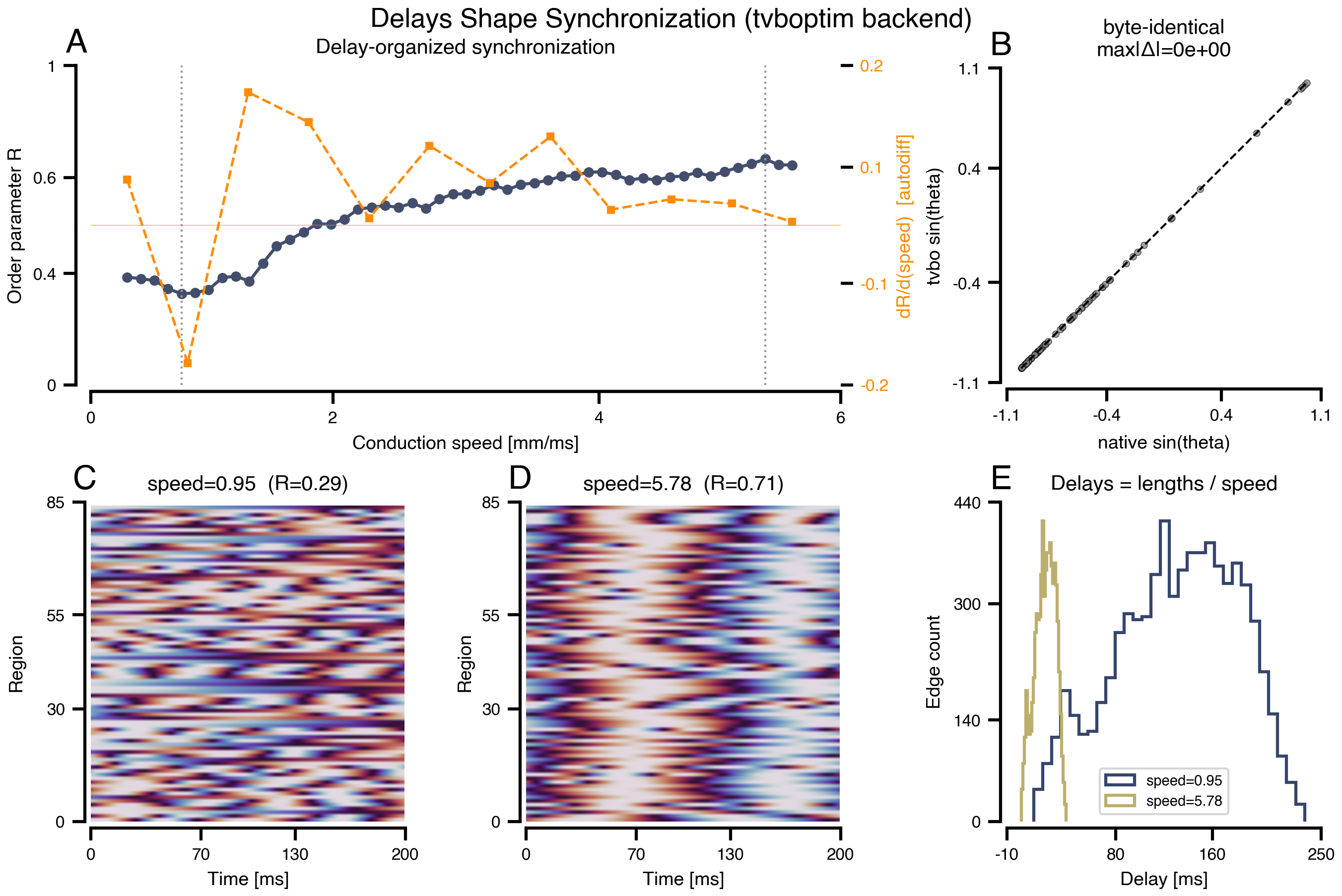
The conduction speed enters as a single DenseLengthGraph.speed leaf, so the very same declarative model is both sweepable (panel A, blue, via exp.run(mode="exploration")) and differentiable (panel A, orange, by jax.grad through delays = lengths / speed once history_interpolation="linear" is enabled). Panel B confirms the tvbo-generated code reproduces a hand-written native tvboptim run bit-for-bit.
References
- Petkoski, S. & Jirsa, V. K. (2019). Transmission time delays organize the brain network synchronization. Phil. Trans. R. Soc. A 377, 20180132.
- Yeung, M. K. S. & Strogatz, S. H. (1999). Time delay in the Kuramoto model of coupled oscillators. Phys. Rev. Lett. 82, 648.