Automatic Higher-Order ODE Lowering

Symbolic round-trip between SymPy and ModelingToolkit.jl

Why this matters

Many dynamical systems are naturally expressed as higher-order ODEs, but most simulation backends only support first-order systems. Manually rewriting \(\ddot{x} = f(x)\) into a first-order system is tedious and error-prone — you need to introduce auxiliary variables, track extra initial conditions, and keep everything consistent.

tvbo automates this by round-tripping through ModelingToolkit.jl: send a higher-order system to Julia, let MTK’s compiler do the structural transformation, and get back clean first-order symbolic equations ready for any backend.

\[ \ddot{x} = \sigma(y - x) \quad \Longrightarrow \quad \begin{cases} \dot{x} = x_t \\ \dot{x_t} = \sigma(y - x) \end{cases} \]

The YAML Specification

Mark a state variable with equation_order: 2 to declare its equation as second-order. Provide the derivative initial condition separately with derivative_initial_value: 2.0:

state_variables:
  x:
    name: x
    initial_value: 1.0
    derivative_initial_value: 2.0
    equation_order: 2
    equation:
      rhs: sigma * (y - x)

Step 1: Load and Inspect the SymPy Equations

from tvbo import SimulationExperiment
from IPython.display import Markdown
exp = SimulationExperiment.from_file(
    "yaml/lorenz_higher_order.yaml"
)
Markdown(exp.dynamics.generate_report(derivative_notation='dot'))

Lorenz63_HigherOrder

Second-order Lorenz variant from the MTK documentation. Variable x has equation_order=2, so d²x/dt² = σ(y-x).

State Equations

\[ \ddot{x} = \sigma*\left(y - x\right) \] \[ \dot{y} = - y + x*\left(\rho - z\right) \] \[ \dot{z} = x*y - \beta*z \]

Parameters

Parameter	Value	Unit	Description
\(\beta\)	2.6666666666666665	N/A	Geometric factor (8/3)
\(\rho\)	28.0	N/A	Rayleigh number
\(\sigma\)	10.0	N/A	Prandtl number

tvbo correctly represents the second-order derivative

Step 2: Render MTK Code

code = exp.render_code("mtk")
print(code)






using ModelingToolkit
using ModelingToolkit: t_nounits as t, D_nounits as Dt
using OrdinaryDiffEqTsit5


@component function Lorenz63_HigherOrder(; name)
    @parameters begin
        beta = 2.6666666666666665, [description="Geometric factor (8/3)"]
        rho = 28.0, [description="Rayleigh number"]
        sigma = 10.0, [description="Prandtl number"]
    end
    @variables begin
        x(t)=1.0, [description="Second-order state variable. The equation x'' = σ(y - x) is automatically lowered to two first-order equations by MTK."]
        y(t)=0.0, [description="Temperature difference (horizontal)"]
        z(t)=0.0, [description="Temperature difference (vertical)"]
    end
    eqs = [
        Dt(Dt(x)) ~ sigma * (y - x),
        Dt(y) ~ -y + x * (rho - z),
        Dt(z) ~ x * y - beta * z,
    ]
    return System(eqs, t; name, checks=false)
end

@named sys_model = Lorenz63_HigherOrder()
sys = mtkcompile(sys_model)

u0 = [Dt(sys.x) => 2.0]

tspan = (0.0, 100.0)
prob = ODEProblem(sys, u0, tspan, jac=true)
sol = solve(prob, Tsit5(); saveat=0.01)

using Plots
plot(sol; title="Lorenz63_HigherOrder")

The template generates Dt(Dt(x)) — MTK’s notation for \(\frac{d^2 x}{dt^2}\)

The derivative initial condition is passed via:

u0 = [Dt(sys.x) => 2.0]

Step 3: Symbolic Round-Trip — Get Lowered Equations

Here is the key feature: we send the higher-order system to Julia, let MTK’s mtkcompile do the structural transformation, and extract the lowered first-order equations back as SymPy.

from tvbo.adapters.modelingtoolkit import ModelingToolkitAdapter

adapter = ModelingToolkitAdapter()
firstorder_ODE = adapter.lower(exp.dynamics)
Markdown(firstorder_ODE.generate_report())

Detected IPython. Loading juliacall extension. See https://juliapy.github.io/PythonCall.jl/stable/compat/#IPython

Lorenz63_HigherOrder_FirstOrder

First-order equivalent of Lorenz63_HigherOrder (lowered via MTK).

State Equations

\[ \dot{x} = x_{t} \] \[ \dot{y} = - y + x*\left(\rho - z\right) \] \[ \dot{z} = x*y - \beta*z \] \[ \dot{x_{t}} = \sigma*\left(y - x\right) \]

Parameters

Parameter	Value	Unit	Description
\(\beta\)	2.6666666666666665	N/A	Geometric factor (8/3)
\(\rho\)	28.0	N/A	Rayleigh number
\(\sigma\)	10.0	N/A	Prandtl number

To run the lowered system with backends that only support first-order ODEs:

lowered_exp = adapter.lower(exp)
lowered_exp.integration.method='Heun'
result = lowered_exp.run("tvboptim")
result.integration.to_timeseries().get_state(["x", "y"]).plot(type="statespace")


============================================================
STEP 1: Running simulation...
============================================================
  Simulation period: 100.0 ms, dt: 0.01 ms
  Transient period: 0.0 ms
  Simulation complete.

============================================================
Experiment complete.
============================================================

MTK introduced x_t (written as xˍt in Julia) and produced four first-order equations:

The returned SymPy equations are standard sympy.Eq objects — they can be used for further symbolic analysis, code generation to other backends, or substitution.

Step 4: Run the Simulation

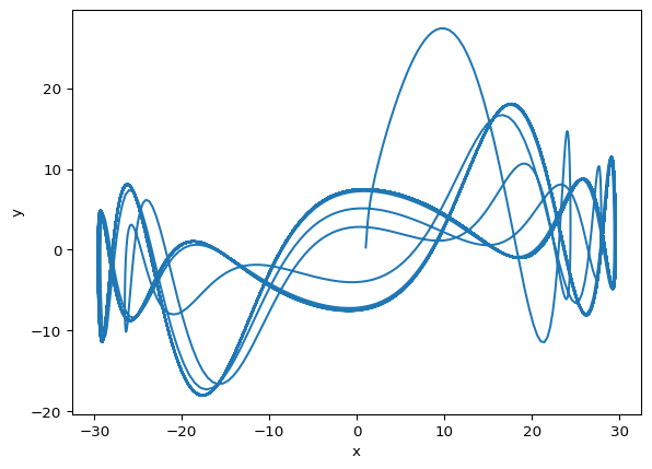
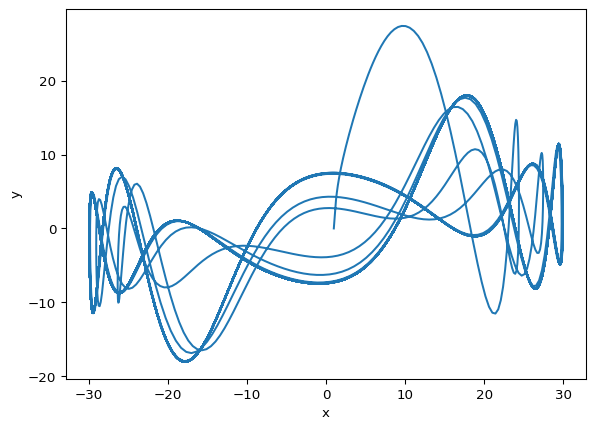
result = exp.run("mtk")
result.get_state(["x", "y"]).plot(type="statespace")

This matches the original MTK tutorial’s \(x\)-\(y\) state-space plot.

Summary

Step	What happens
YAML	Define `equation_order: 2` on the state variable
tvbo → MTK	Generates `Dt(Dt(x)) ~ sigma * (y - x)`
MTK compiles	Introduces \(x_t\), produces first-order system
MTK → tvbo	Extracts lowered equations as SymPy
Run anywhere	Lowered system works with `tvboptim`, `JAX`, `TVB`, …