from tvbo import Dynamics
import matplotlib.pyplot as plt

LIN_YAML = """
name: LinearScalar
description: |
  Scalar linear ODE $\\dot x = a x$. Stability of the origin is governed by
  the sign of $a$.
parameters:
  a:
    name: a
    value: 1.0
state_variables:
  x:
    name: x
    domain: { lo: -5.0, hi: 5.0 }
    equation:
      lhs: Derivative(x, t)
      rhs: a*x
    initial_value: 1.0
"""1. Linear Stability
“The simplest dynamical system is also the most fundamental: its qualitative behaviour is governed by a single number.”
The starting point of bifurcation theory is the scalar linear ODE:
\[ \dot x(t) = a\,x(t), \qquad x(0) = x_0, \]
with closed-form solution \(x(t) = x_0\,e^{a\,t}\).
- State variable \(x(t)\): the unknown.
- Initial condition \(x_0\): fixes the trajectory.
- Parameter \(a\): the stability indicator.
Three regimes follow from the sign of \(a\):
| \(a\) | Eigenvalue | Equilibrium \(x = 0\) | Trajectories |
|---|---|---|---|
| \(a < 0\) | real, negative | stable node | exponential decay \(x_0\,e^{-|a|t} \to 0\) |
| \(a = 0\) | zero | non-hyperbolic | \(x(t) \equiv x_0\) |
| \(a > 0\) | real, positive | unstable node | exponential growth \(x_0\,e^{+|a|t} \to \infty\) |
The line \(a = 0\) is the simplest example of a bifurcation — the qualitative phase portrait changes there.
We define the system inline as a TVBO Dynamics. Only the YAML changes; all plotting calls are TVBO standard library:
A family of solutions across \(a\)
Five values of \(a\) from strongly damped to strongly amplified, all started at \(x_0 = 1\) and integrated for 4 time units. Axis limits match the legacy slide (ExpExample0Red.png).
import numpy as np
fig, ax = plt.subplots(figsize=(5, 4))
for a, color in zip([-1.0, -0.5, 0.0, 0.5, 1.0], ["C0", "C1", "0.4", "C2", "C3"]):
    dyn = Dynamics.from_string(LIN_YAML)
    dyn.parameters["a"].value = a
    dyn.plot("x", duration=4, dt=1e-3, ax=ax)
    ax.lines[-1].set_color(color)
    ax.lines[-1].set_label(f"$a = {a:+.1f}$")
ax.set_xlabel("Time $t$"); ax.set_ylabel("$x(t)$")
ax.set_xlim(0, 4); ax.set_ylim(-0.2, 4.0)
ax.legend(handlelength=1, loc="upper left")
plt.tight_layout(); plt.show()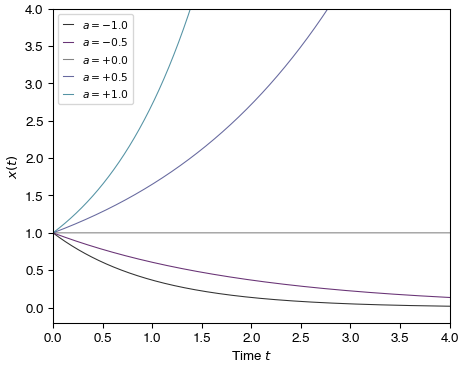
The slope of every curve at \(t = 0\) equals \(a\) (compare \(\dot x(0) = a\,x_0\)); its sign decides whether the trajectory grows or decays. This is the eigenvalue criterion in its simplest form.
Reproducing ExpExamplePert.png
Same system, but starting from a tiny perturbation \(\delta = 10^{-6}\) applied at \(t = 1\). The qualitative behaviour is identical to the un-perturbed case: the only information that survives a small perturbation of an unstable trajectory is the sign of \(a\). This motivates the local-flow / linearisation viewpoint explored in the next section.
tv = np.linspace(0, 4, 1000)
n4 = tv.size // 4
delta = 1e-6
x_pos = np.zeros_like(tv); x_pos[n4:] = delta * np.exp(tv[n4:] - tv[n4])
x_neg = np.zeros_like(tv); x_neg[n4:] = delta * np.exp(-(tv[n4:] - tv[n4]))

fig, ax = plt.subplots(figsize=(5, 4))
ax.axhline(0, color="#c9211e", linestyle="--")
ax.plot(tv, x_pos, color="C0", lw=2, label="$a=+1$ (unstable)")
ax.plot(tv, x_neg, color="C1", lw=2, label="$a=-1$ (stable)")
ax.set_xlabel("Time $t$"); ax.set_ylabel("$x(t)$")
ax.set_xlim(0, 4); ax.set_ylim(-0.2 * 1e-5 / 4, 1e-5)
ax.legend(handlelength=1)
plt.tight_layout(); plt.show()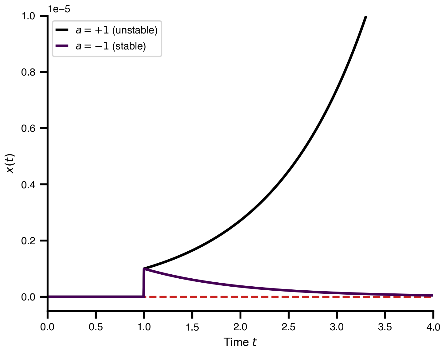
Linking to the next section
For nonlinear systems \(\dot x = f(x)\), linear stability of an equilibrium \(x^*\) is decided by the eigenvalues of the Jacobian \(J = \partial f / \partial x \,\big|_{x = x^*}\). The 1-D linear ODE above is just the special case \(f(x) = a\,x\) with \(J \equiv a\); everything else is a multidimensional generalisation. The next chapter shows the canonical 2-D classification (node / saddle / focus / centre) directly from YAML.