Network Diffusion

Getting started with NetworkDynamics.jl via tvbo

Replicates the NetworkDynamics.jl Getting Started tutorial — diffusion on an undirected network with 20 nodes. A single scalar state per node, antisymmetric diffusive coupling, and convergence to equilibrium.

YAML Specification

# =============================================================================
# Network Diffusion - Getting Started with NetworkDynamics.jl
# =============================================================================
# Source: https://juliadynamics.github.io/NetworkDynamics.jl/stable/generated/getting_started_with_network_dynamics/
#
# Diffusion on an undirected network. Each node state evolves as the sum of
# incoming edge flows.
# Vertex has no intrinsic dynamics; edge is antisymmetric: e = v_src - v_dst.
# =============================================================================

id: 100
label: "Network Diffusion"
description: >
    Diffusion on an undirected network.  Each node state evolves as the sum
    of incoming edge flows.  The edge computes the antisymmetric difference
    between source and destination states: e = v_src - v_dst.
    Recreates the NetworkDynamics.jl Getting Started tutorial.
references:
    - "https://juliadynamics.github.io/NetworkDynamics.jl/stable/generated/getting_started_with_network_dynamics/"

# -- Local Dynamics ------------------------------------------------------------
dynamics:
    name: Diffusion
    label: "Diffusion vertex"
    description: >
        Node with no internal dynamics.  The rate of change of the single
        state variable v equals the aggregated incoming edge flow (esum).
        Corresponds to the discrete Laplacian: dx_i = sum_j A_ji (x_j - x_i).
    system_type: continuous
    autonomous: true
    parameters: {}
    coupling_terms:
        c_flow:
            description: "Aggregated edge flow into this vertex (sum of incident edge outputs)"
    state_variables:
        v:
            label: "Diffusion state"
            description: "Abstract quantity (e.g. temperature, concentration) diffusing on the network"
            equation:
                rhs: "c_flow"
            initial_value: 0.0
            distribution:
                name: Gaussian
                seed: 1
                domain: { lo: -3.0, hi: 3.0 }
            variable_of_interest: true

# -- Network -------------------------------------------------------------------
network:
    label: "20-node Barabási-Albert network"
    description: >
        Undirected Barabási-Albert scale-free random graph with 20 nodes
        and average degree 4.  Matches the original tutorial.
    number_of_nodes: 20
    graph_generator:
        name: barabasi_albert
        type: BarabasiAlbert
        parameters:
            k: { name: k, value: 4 }
    coupling:
        DiffusiveCoupling:
            name: DiffusiveCoupling
            label: "Diffusive Coupling"
            description: >
                Antisymmetric edge function: output is the difference between
                source and destination vertex states.
                g_dst(v_src, v_dst) = v_src - v_dst;
                g_src(v_src, v_dst) = v_dst - v_src (by AntiSymmetric wrapper).
            delayed: false
            pre_expression:
                rhs: "x_j - x_i"
                description: "Discrete gradient: source state minus destination state"

# -- Integration ---------------------------------------------------------------
integration:
    description: "Explicit Runge-Kutta (Tsit5) with dt=0.01 over t in [0, 2]"
    method: Tsit5
    step_size: 0.01
    duration: 2.0
    time_scale: "a.u."

Model Report

Network Diffusion

Diffusion on an undirected network. Each node state evolves as the sum of incoming edge flows. The edge computes the antisymmetric difference between source and destination states: e = v_src - v_dst. Recreates the NetworkDynamics.jl Getting Started tutorial.

1. Brain Network: 20-node Barabási-Albert network

Undirected Barabási-Albert scale-free random graph with 20 nodes and average degree 4. Matches the original tutorial.

Regions: 20

Coupling: Diffusive Coupling

Antisymmetric edge function: output is the difference between source and destination vertex states. g_dst(v_src, v_dst) = v_src - v_dst; g_src(v_src, v_dst) = v_dst - v_src (by AntiSymmetric wrapper).

Pre-synaptic: \(c_{\text{pre}} = x_{j} - x_{i}\)

2. Local Dynamics: Diffusion vertex

Node with no internal dynamics. The model comprises 1 state variables.

2.1 State Equations

\[\dot{v} = c_{flow}\]

2.2 Parameters

Parameter	Value	Unit	Description

3. Numerical Integration

Method: Tsit5
Time step: \(\Delta t = 0.01\) ms
Duration: 2.0 ms

References

https://juliadynamics.github.io/NetworkDynamics.jl/stable/generated/getting_started_with_network_dynamics/

Generated Julia Code

from tvbo import SimulationExperiment
exp = SimulationExperiment.from_file("yaml/diffusion.yaml")
Code(exp.render_code("networkdynamics"), language='julia')

using Graphs
using NetworkDynamics

using OrdinaryDiffEqTsit5







function Diffusion_f!(dx, x, esum, p, t)
    v = x[1]

    c_flow = esum[1]
    dx[1] = c_flow
    nothing
end

vertex_Diffusion = VertexModel(;
    f = Diffusion_f!,
    g = StateMask(1:1),
    sym = [:v],
    name = :Diffusion,
)








function DiffusiveCoupling_edge_g!(e_dst, v_src, v_dst, p, t)
    e_dst[1] = v_src[1] - v_dst[1]
    nothing
end

edge_DiffusiveCoupling = EdgeModel(;
    g = AntiSymmetric(DiffusiveCoupling_edge_g!),
    outsym = [:coupling],
    name = :DiffusiveCoupling,
)




g = barabasi_albert(20, 4)


nw = Network(g, vertex_Diffusion, edge_DiffusiveCoupling)




s = NWState(nw)
using Random
rng = MersenneTwister(1)

for node in 1:nv(g)
    s.v[node, :v] = (-3.0 + 3.0) / 2 .+ (3.0 - -3.0) / 6 .* randn(rng)
end



tspan = (0.0, 2.0)
prob = ODEProblem(nw, uflat(s), tspan, pflat(s))
sol = solve(prob, Tsit5(); saveat=0.01)

adj_matrix = Float64.(adjacency_matrix(g))

using Random: MersenneTwister
function spring_layout(g; seed=42, iterations=50, k=1.0)
    rng = MersenneTwister(seed)
    n = nv(g)
    pos = randn(rng, n, 2)
    for _ in 1:iterations
        disp = zeros(n, 2)
        for i in 1:n, j in (i+1):n
            d = pos[i, :] - pos[j, :]
            dist = max(norm(d), 0.01)
            rep = k^2 / dist
            disp[i, :] .+= d / dist * rep
            disp[j, :] .-= d / dist * rep
        end
        for e in edges(g)
            i, j = src(e), dst(e)
            d = pos[j, :] - pos[i, :]
            dist = max(norm(d), 0.01)
            att = dist^2 / k
            disp[i, :] .+= d / dist * att
            disp[j, :] .-= d / dist * att
        end
        for i in 1:n
            dl = max(norm(disp[i, :]), 0.01)
            pos[i, :] .+= disp[i, :] / dl * min(dl, 0.1)
        end
    end
    return pos
end
using LinearAlgebra: norm
node_positions = spring_layout(g)

using Plots
plot(sol; ylabel="state", xlabel="time", title="Diffusion on 20-node network")

Run & Plot

ts = exp.run(format="networkdynamics")
ts.plot()

Detected IPython. Loading juliacall extension. See https://juliapy.github.io/PythonCall.jl/stable/compat/#IPython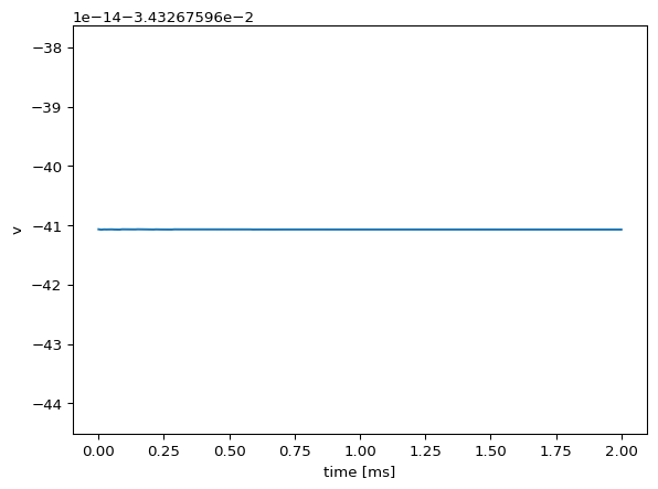

Results

Shape: (201, 1, 20)
Time range: 0.0 – 2.0
Final state std: 0.003375
(Should converge to ~0 as all nodes reach equilibrium)

Animate

ani = ts.animate("v", format="dots")
ani.save("_output/diffusion.gif", writer="pillow", fps=20)