TVB Connectome Round-Trip

Lossless import/export between TVB and tvbo — connectivity, surfaces, and HDF5 persistence

TVB (The Virtual Brain) stores brain connectivity as Connectivity objects with weights, tract lengths, centres, region labels, and conduction speed. TVBO can import these losslessly, persist them as YAML + HDF5, and export back to TVB with identical arrays.

import numpy as np
import tempfile
from pathlib import Path
from tvbo import Network
from bsplot.surface import plot_surf
from bsplot.graph import create_network

1. Import TVB Connectivity

Load the default TVB connectivity (76-region Hagmann parcellation) and convert it to a tvbo Network:

from tvb.datatypes.connectivity import Connectivity

conn = Connectivity.from_file()
conn.configure()

print(f"TVB: {conn.weights.shape[0]} regions, "
      f"speed = {conn.speed[0]} mm/ms")

TVB: 76 regions, speed = 3.0 mm/ms

net = Network.from_tvb(conn)

print(f"tvbo: {net.number_of_nodes} nodes")
print(f"Label: {net.label}")
print(f"Conduction speed: {net.conduction_speed.value} {net.conduction_speed.unit}")
print(f"Weights range: [{net.weights_matrix.min():.4f}, {net.weights_matrix.max():.4f}]")
print(f"Lengths range: [{net.lengths_matrix.min():.1f}, {net.lengths_matrix.max():.1f}] mm")

tvbo: 76 nodes
Label: Connectivity gid: 9df860e7-5404-4cf5-98d7-500e11dfbbed
Conduction speed: 3.0 mm_per_ms
Weights range: [0.0000, 3.0000]
Lengths range: [0.0, 153.5] mm

All TVB per-node metadata is preserved — cortical flags, areas, hemispheres, and orientations:

node0 = net.nodes[0]
print(f"Node 0: {node0.label}")
print(f"  Position: ({node0.position.x:.1f}, {node0.position.y:.1f}, {node0.position.z:.1f})")
if node0.parameters:
    params = node0.parameters
    for name in ["cortical", "area", "hemisphere"]:
        p = getattr(params, name, None)
        if p is not None:
            print(f"  {name}: {p.value}")

Node 0: rA1
  Position: (-9.9, -47.1, -3.1)

2. Visualize the Connectome

net.plot_matrix()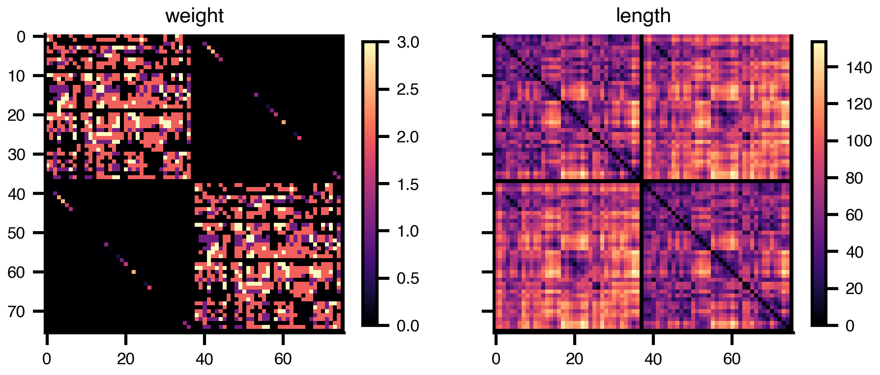

Figure 1: Weight matrix of the TVB default connectivity (76 regions)

net.plot_overview(plot_brain=False)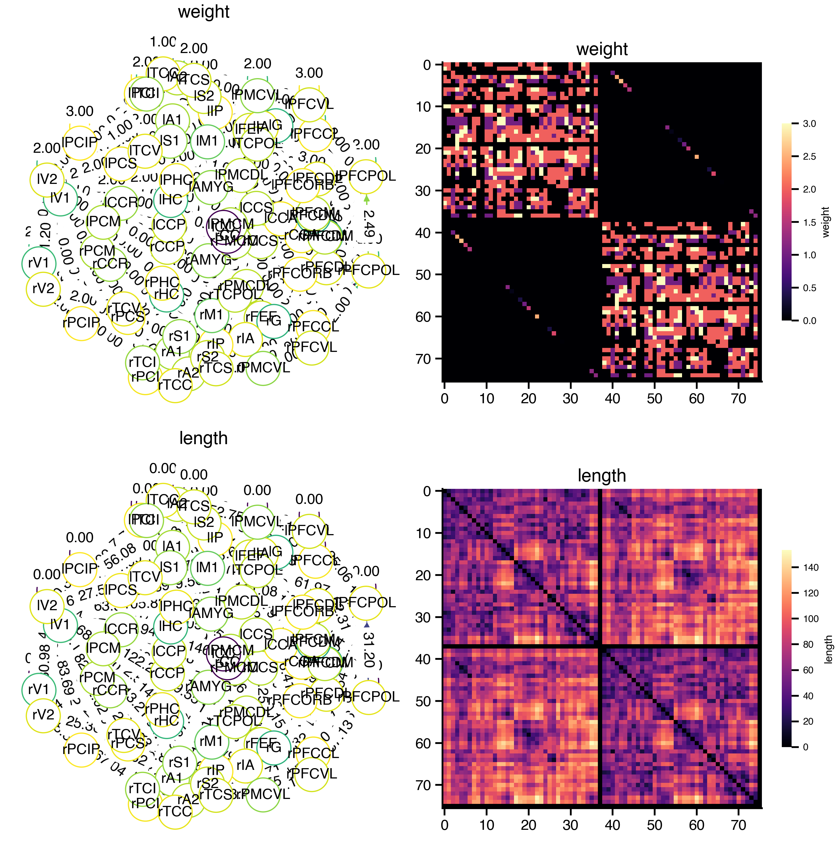

Figure 2: Network overview — weights, lengths, and graph layout

3. Save as YAML + HDF5

TVBO stores networks as a human-readable YAML sidecar (metadata and schema) plus an HDF5 companion file (dense matrix data with gzip compression).

outdir = Path(tempfile.mkdtemp())
yaml_path = outdir / "tvb_default_76.yaml"

net.save(yaml_path)

print("Created files:")
for f in sorted(outdir.iterdir()):
    sz = f.stat().st_size
    print(f"  {f.name:30s}  ({sz:,} bytes)")

Created files:
  tvb_default_76.h5               (64,256 bytes)
  tvb_default_76.yaml             (15,549 bytes)

The YAML sidecar is fully self-describing:

# Show first 40 lines of the sidecar
lines = yaml_path.read_text().splitlines()
for line in lines[:40]:
    print(line)
print(f"... ({len(lines)} lines total)")

tvbo_class: tvbo:Network
schema_version: tvb-datamodel/0.7.0
label: 'Connectivity gid: 9df860e7-5404-4cf5-98d7-500e11dfbbed'
number_of_nodes: 76
descriptor: SC
distance_unit: mm
time_unit: ms
data_file: tvb_default_76.h5
parameters:
  conduction_speed:
    label: v
    value: 3.0
    unit: mm_per_ms
nodes:
- id: 0
  label: rA1
  parameters:
    cortical:
      value: 1.0
    area:
      value: 396.44065
    hemisphere:
      value: 1.0
  position:
    x: -9.885591
    y: -47.084818
    z: -3.13936
- id: 1
  label: rA2
  parameters:
    cortical:
      value: 1.0
    area:
      value: 937.50289
    hemisphere:
      value: 1.0
  position:
    x: -2.605247
    y: -55.324507
    z: -7.065423
... (1015 lines total)

4. Reload and Verify

reloaded = Network.from_file(yaml_path)

print(f"Reloaded: {reloaded.number_of_nodes} nodes")
print(f"Label: {reloaded.label}")

Reloaded: 76 nodes
Label: Connectivity gid: 9df860e7-5404-4cf5-98d7-500e11dfbbed

Verify lossless round-trip — arrays match exactly:

np.testing.assert_allclose(reloaded.weights_matrix, net.weights_matrix)
np.testing.assert_allclose(reloaded.lengths_matrix, net.lengths_matrix)
print("✓ Weights match")
print("✓ Lengths match")

✓ Weights match
✓ Lengths match

Node metadata also survives:

for i in range(min(5, net.number_of_nodes)):
    orig = net.nodes[i]
    load = reloaded.nodes[i]
    assert orig.label == load.label, f"Label mismatch at node {i}"
    assert abs(orig.position.x - load.position.x) < 1e-6
print(f"✓ First {min(5, net.number_of_nodes)} node labels and positions match")

✓ First 5 node labels and positions match

5. Export Back to TVB

Convert the reloaded network back to a TVB Connectivity and compare with the original:

conn2 = reloaded.execute(format="tvb")

print(f"TVB round-trip: {conn2.weights.shape[0]} regions")
np.testing.assert_allclose(conn2.weights, conn.weights)
np.testing.assert_allclose(conn2.tract_lengths, conn.tract_lengths)
np.testing.assert_allclose(conn2.centres, conn.centres, atol=1e-5)
np.testing.assert_allclose(conn2.speed, conn.speed)
print("✓ weights identical")
print("✓ tract_lengths identical")
print("✓ centres identical (atol=1e-5)")
print(f"✓ speed identical ({conn2.speed[0]} mm/ms)")

TVB round-trip: 76 regions
✓ weights identical
✓ tract_lengths identical
✓ centres identical (atol=1e-5)
✓ speed identical (3.0 mm/ms)

Centre coordinates

import matplotlib.pyplot as plt

fig, axes = plt.subplots(1, 3, figsize=(12, 3.5))
for ax, (dim, lbl) in zip(axes, enumerate(["x (mm)", "y (mm)", "z (mm)"])):
    orig = conn.centres[:, dim]
    rt = conn2.centres[:, dim]
    ax.scatter(orig, rt, s=8, alpha=0.7)
    lims = [min(orig.min(), rt.min()) - 2, max(orig.max(), rt.max()) + 2]
    ax.plot(lims, lims, 'k--', lw=0.8, alpha=0.5)
    ax.set_xlim(lims); ax.set_ylim(lims)
    ax.set_xlabel(f"Original {lbl}"); ax.set_ylabel(f"Round-trip {lbl}")
    ax.set_aspect('equal')
fig.suptitle("Centre coordinates: original vs round-trip", fontsize=11)
plt.tight_layout()
plt.show()
print(f"Max centre deviation: {np.abs(conn2.centres - conn.centres).max():.2e} mm")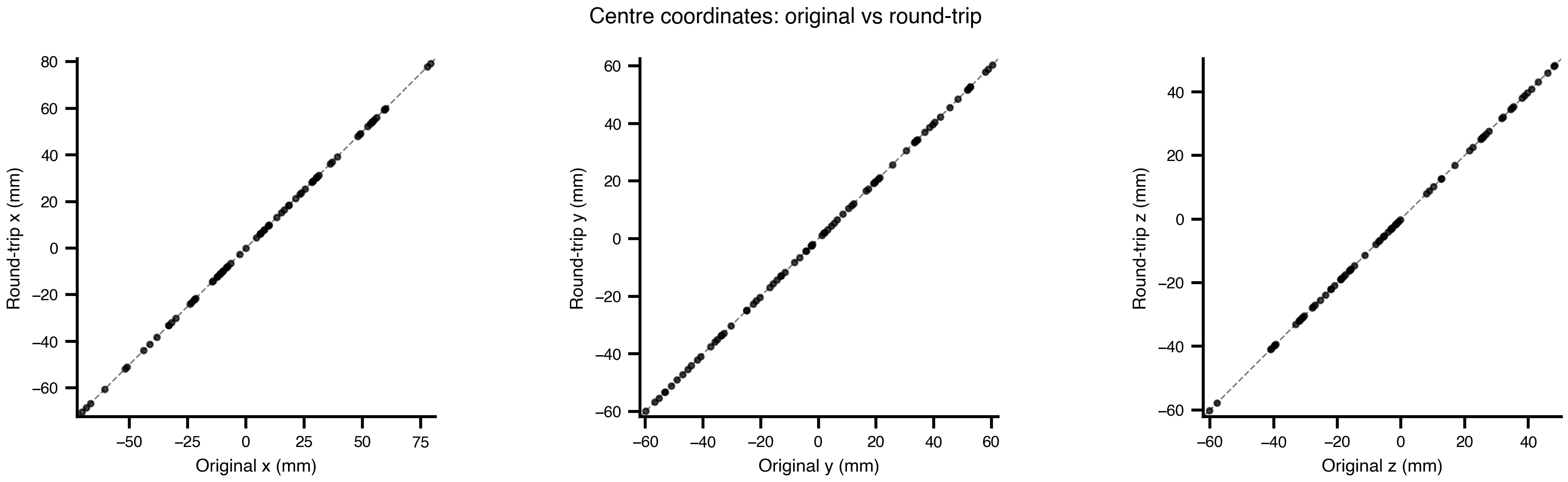

Max centre deviation: 0.00e+00 mm

diff = conn2.weights - conn.weights
fig, ax = plt.subplots(figsize=(6, 5))
im = ax.imshow(diff, cmap="RdBu_r", vmin=-1e-10, vmax=1e-10)
ax.set_title("Weight difference (original − round-trip)")
ax.set_xlabel("Region")
ax.set_ylabel("Region")
fig.colorbar(im, ax=ax, label="Δweight")
plt.tight_layout()
plt.show()
print(f"Max absolute difference: {np.abs(diff).max():.2e}")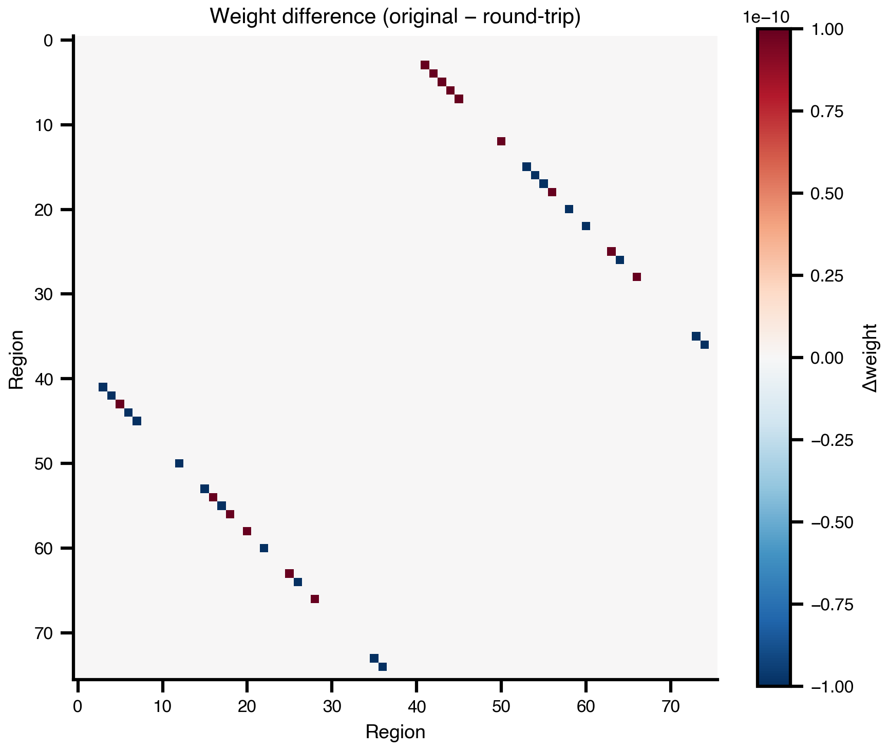

Figure 3: Difference between original and round-tripped weights (should be zero everywhere)

Max absolute difference: 1.18e-07

6. Surface Network (Multi-Level)

TVB surface simulations use three objects: Connectivity (regions), CorticalSurface (mesh), and RegionMapping (vertex → region). TVBO imports all three into a linked pair of networks.

from tvb.datatypes.surfaces import CorticalSurface
from tvb.datatypes.region_mapping import RegionMapping

surf = CorticalSurface.from_file()
surf.configure()

rmap = RegionMapping.from_file()
rmap.connectivity = conn
rmap.surface = surf
rmap.configure()

print(f"Surface: {surf.vertices.shape[0]} vertices, "
      f"{surf.triangles.shape[0]} triangles")
print(f"Region mapping: {rmap.array_data.shape[0]} entries → "
      f"{len(np.unique(rmap.array_data))} regions")

Surface: 16384 vertices, 32760 triangles
Region mapping: 16384 entries → 76 regions

region_net, surface_net = Network.from_tvb_surface(conn, surf, rmap)

print(f"Region network:  {region_net.number_of_nodes} nodes")
print(f"Surface network: {surface_net.number_of_nodes} nodes")
print(f"Mesh: {surface_net.mesh.number_of_vertices} vertices, "
      f"{surface_net.mesh.number_of_elements} triangles")
print(f"Parent link: {surface_net.parent_network is not None}")

Region network:  76 nodes
Surface network: 16384 nodes
Mesh: 16384 vertices, 32760 triangles
Parent link: True

Visualize the Cortical Mesh

vertices = surface_net._mesh_vertices
triangles = surface_net._mesh_elements
region_ids = surface_net.node_mapping_data.astype(float)

fig, axes = plt.subplots(1, 2, figsize=(10, 5))

plot_surf(
    vertices=vertices, faces=triangles, overlay=region_ids,
    view='lateral', cmap='tab20', parcellated=True, ax=axes[0],
)
axes[0].set_title("Lateral")

plot_surf(
    vertices=vertices, faces=triangles, overlay=region_ids,
    view='dorsal', cmap='tab20', parcellated=True, ax=axes[1],
)
axes[1].set_title("Dorsal")

plt.tight_layout()
plt.show()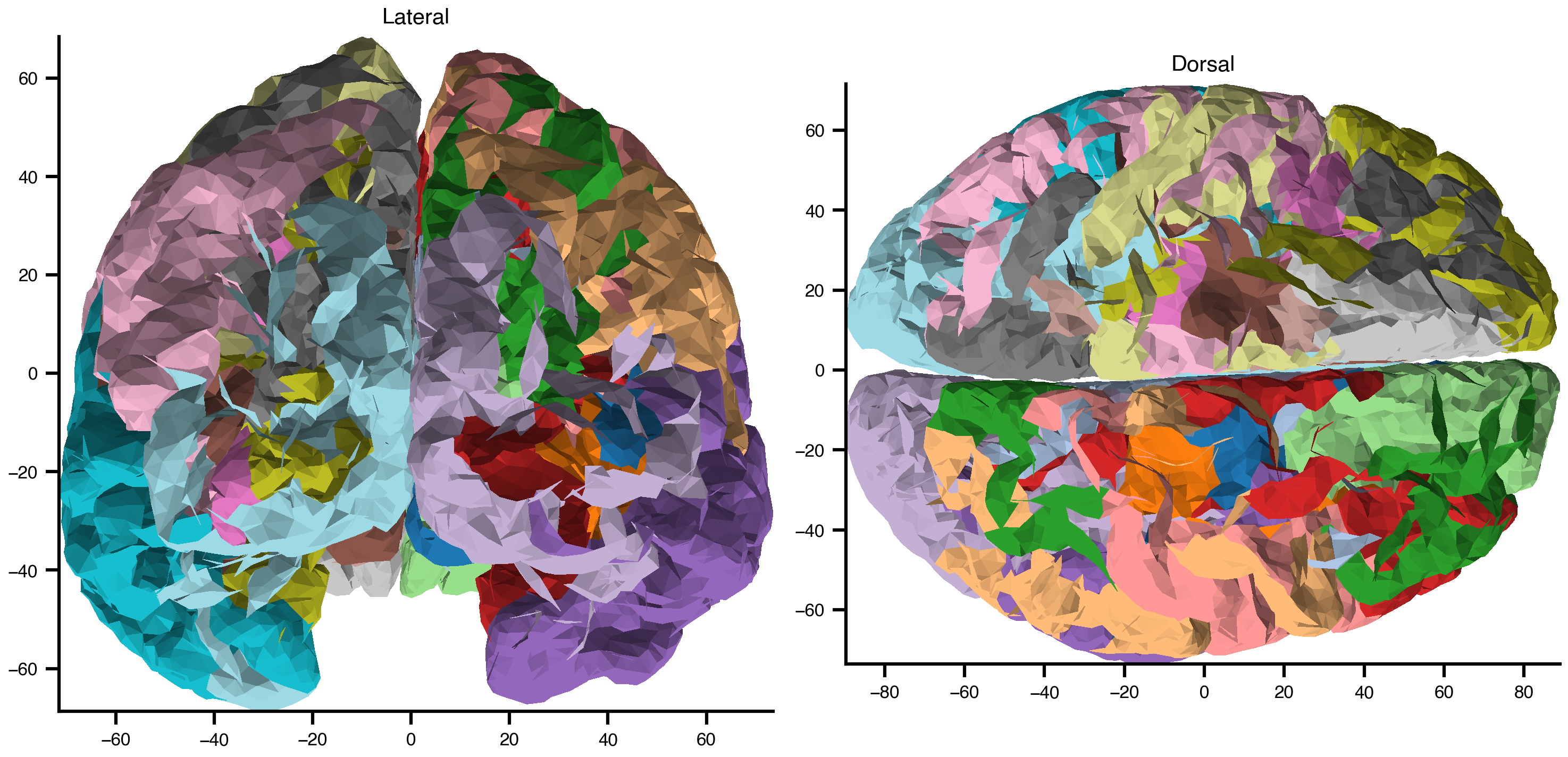

Figure 4: TVB default cortical surface coloured by region assignment

Save and Reload Multi-Level Networks

surf_dir = Path(tempfile.mkdtemp())

region_net.save(surf_dir / "regions.yaml")
surface_net.save(surf_dir / "surface.yaml")

print("Surface network files:")
for f in sorted(surf_dir.iterdir()):
    sz = f.stat().st_size
    print(f"  {f.name:30s}  ({sz:,} bytes)")

Surface network files:
  regions.h5                      (64,256 bytes)
  regions.yaml                    (15,542 bytes)
  surface.h5                      (823,061 bytes)
  surface.yaml                    (2,002,533 bytes)

reloaded_surf = Network.from_file(surf_dir / "surface.yaml")

print(f"Reloaded: {reloaded_surf.number_of_nodes} nodes")
print(f"Mesh vertices: {reloaded_surf._mesh_vertices.shape}")
print(f"Mesh triangles: {reloaded_surf._mesh_elements.shape}")

np.testing.assert_allclose(reloaded_surf._mesh_vertices, vertices)
np.testing.assert_allclose(reloaded_surf._mesh_elements, triangles)
print("✓ Mesh data survives HDF5 round-trip")

Reloaded: 16384 nodes
Mesh vertices: (16384, 3)
Mesh triangles: (32760, 3)
✓ Mesh data survives HDF5 round-trip

Optional: MNE Projection Layer in the Network Section

The MNE exporter creates a sensor-to-region projection network in tvbo format (sensors_eeg_standard1005_fsaverage_aparc_projection.yaml). This can be handled in the same multi-layer network workflow as other network resources.

from tvbo import database_path

mne_yaml = (
    database_path
    / "networks"
    / "sensors_eeg_standard1005_fsaverage_aparc_projection.yaml"
)
mne_meta = mne_yaml.with_name(f"{mne_yaml.stem}_plotmeta.npz")

if mne_yaml.exists() and mne_meta.exists():
    mne_net = Network.from_file(mne_yaml)
    mne_gain = np.asarray(mne_net.matrix("gain", format="dense"), dtype=float)
    mne_plotmeta = np.load(mne_meta)

    mne_region_labels = [str(x) for x in mne_plotmeta["region_labels"]]
    mne_region_centers = np.asarray(mne_plotmeta["region_centers_mm"], dtype=float)
    mne_sensor_labels = [str(node.label) for node in mne_net.nodes]
    mne_sensor_pos = np.asarray(
        [[n.position.x, n.position.y, n.position.z] for n in mne_net.nodes],
        dtype=float,
    )

    n_regions = len(mne_region_labels)
    n_sensors = len(mne_sensor_labels)
    n_total = n_regions + n_sensors

    centers = {}
    for i, lbl in enumerate(mne_region_labels):
        centers[f"R:{lbl}"] = tuple(mne_region_centers[i])
    for i, lbl in enumerate(mne_sensor_labels):
        centers[f"S:{lbl}"] = tuple(mne_sensor_pos[i])

    combined = np.zeros((n_total, n_total), dtype=float)
    for i in range(n_sensors):
        for j in range(n_regions):
            combined[n_regions + i, j] = abs(mne_gain[i, j])

    labels = [f"R:{x}" for x in mne_region_labels] + [f"S:{x}" for x in mne_sensor_labels]
    mne_graph = create_network(
        centers,
        {"mne_forward_gain": combined},
        labels=labels,
        threshold_percentile=80,
        directed=True,
        edge_data_key="gain",
    )

    print(
        f"MNE projection layer: nodes={mne_graph.number_of_nodes()}, "
        f"edges={mne_graph.number_of_edges()}, gain_shape={mne_gain.shape}"
    )
else:
    print(
        "MNE projection network not found. Generate it with:\n"
        "python scripts/export_mne_standard1005_projection_network.py"
    )

MNE projection network not found. Generate it with:
python scripts/export_mne_standard1005_projection_network.py

Summary

Step	Method	What It Does
Import	Network.from_tvb(conn)	TVB Connectivity → tvbo Network
Visualize	net.plot_matrix(), net.plot_overview()	Weight/length heatmaps, graph layout
Save	net.save("net.yaml")	YAML sidecar + HDF5 companion
Load	Network.from_file("net.yaml")	Lazy load from file pair
Export	net.execute(format="tvb")	tvbo Network → TVB Connectivity
Surface	Network.from_tvb_surface(conn, surf, rmap)	Multi-level: regions + mesh

The full pipeline is lossless — all matrices, node metadata, mesh geometry, and region mappings survive the round-trip with zero numerical error.