Truncated Backprop-Through-Time (TBPTT) via tvboptim

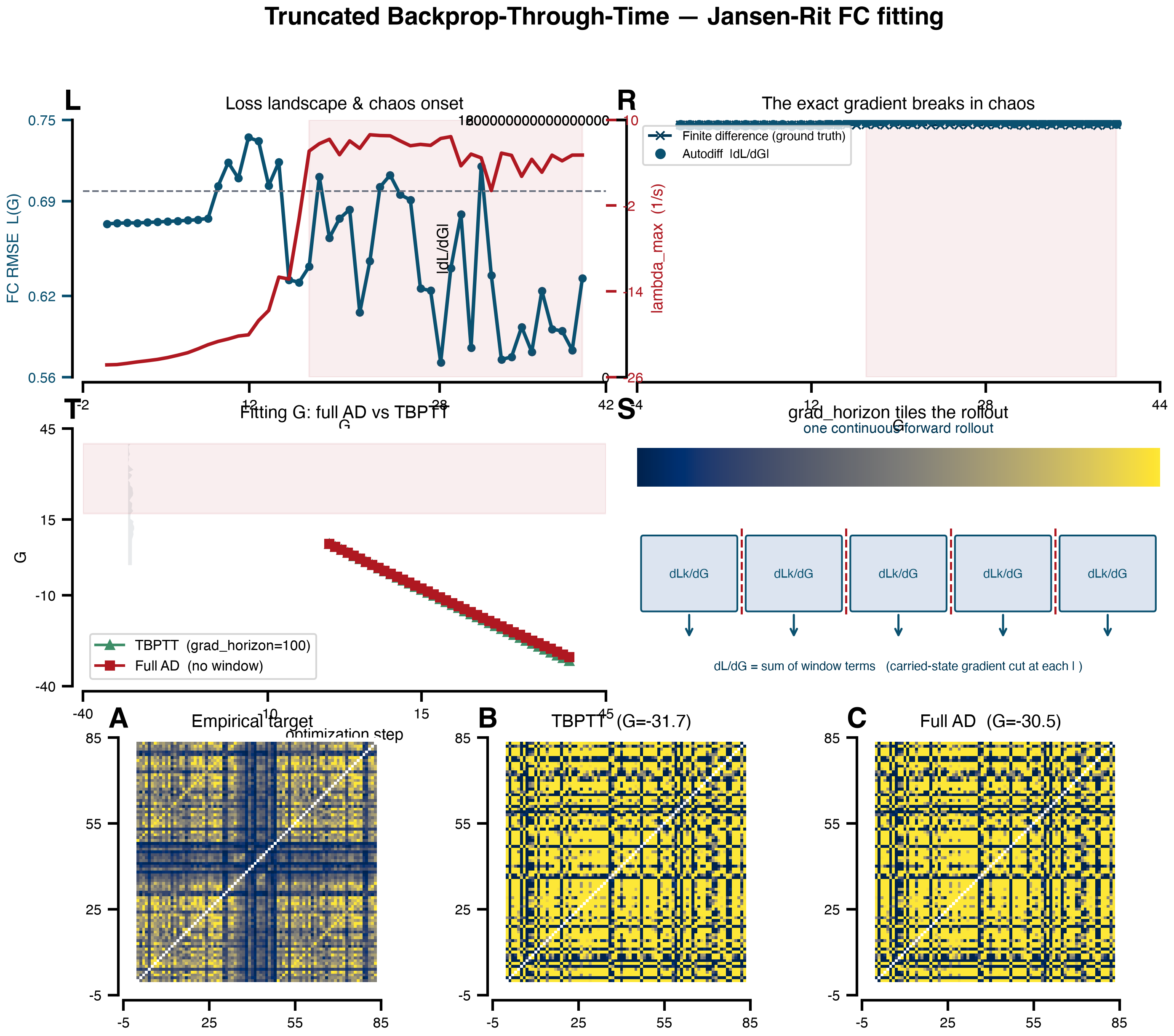
Why the exact FC-loss gradient breaks past the chaos onset, and how a single integration.differentiation window fixes it. Everything below — the diagnostics swept over the global coupling \(G\) (loss, autodiff gradient, finite-difference ground truth, top Lyapunov exponent) and both optimization legs — is derived from one experiment YAML via exp.run; only the plotting is hand-written.

import os

device_count = os.environ.get("TVBO_XLA_DEVICE_COUNT", "8")
os.environ["XLA_FLAGS"] = f"--xla_force_host_platform_device_count={device_count}"

import jax

jax.config.update("jax_enable_x64", True)

from tvbo import SimulationExperiment
from tvbo.datamodel.schema import Differentiation

exp = SimulationExperiment.from_db("TBPTT_JansenRit_FC_Optimization")

# Trim the long production rollout so the page builds in reasonable time. These are
# plain config values on the same YAML — no per-point driver: the diagnostics sweep
# and both descent legs are still computed entirely by exp.run.
exp.integration.duration = 6000.0
exp.integration.transient_time = 1000.0
exp.observations["fc"].pipeline[0].arguments["skip_t"].value = 4  # BOLD samples skipped before FC
exp.optimizations["fit_G"].stages[0].max_iterations = 40

# TBPTT leg: the YAML declares differentiation = {truncation_window: 100, mode: reverse},
# so this run uses Heun(grad_horizon=100) + reverse-mode == truncated BPTT. It also
# computes the motivation sweep (the diagnostics vs G).
tbptt = exp.run("tvboptim", n_G=48)

# Full-AD leg: identical YAML, forward-mode, no truncation window (forward-mode AD
# equals full reverse-mode BPTT for the scalar G — the exact, untruncated gradient).
exp.integration.differentiation = Differentiation(mode="forward")
ad = exp.run("tvboptim", mode="optimization")

============================================================
STEP 1: Running simulation...
============================================================
  Simulation period: 6000.0 ms, dt: 1.0 ms
  Transient period: 1000.0 ms
  Simulation complete.

============================================================
STEP 2: Running explorations...
============================================================
  > G_sweep
  > motivation_sweep
  Explorations complete.

============================================================
STEP 4: Running optimization...
============================================================
Step 0: 0.698428
Step 1: 0.696729
Step 2: 0.695104
Step 3: 0.693510
Step 4: 0.691931
Step 5: 0.690360
Step 6: 0.688795
Step 7: 0.687237
Step 8: 0.685686
Step 9: 0.684144
Step 10: 0.682612
Step 11: 0.681092
Step 12: 0.679585
Step 13: 0.678092
Step 14: 0.676614
Step 15: 0.675151
Step 16: 0.673704
Step 17: 0.672274
Step 18: 0.670859
Step 19: 0.669460
Step 20: 0.668078
Step 21: 0.666711
Step 22: 0.665359
Step 23: 0.664022
Step 24: 0.662700
Step 25: 0.661392
Step 26: 0.660098
Step 27: 0.658817
Step 28: 0.657551
Step 29: 0.656298
Step 30: 0.655059
Step 31: 0.653834
Step 32: 0.652624
Step 33: 0.651428
Step 34: 0.650248
Step 35: 0.649083
Step 36: 0.647936
Step 37: 0.646806
Step 38: 0.645695
Step 39: 0.644603
  Optimization complete.

============================================================
Experiment complete.
============================================================

============================================================
STEP 1: Running simulation...
============================================================
  Simulation period: 6000.0 ms, dt: 1.0 ms
  Transient period: 1000.0 ms
  Simulation complete.

============================================================
STEP 4: Running optimization...
============================================================
Step 0: 0.698428
Step 1: 0.696729
Step 2: 0.695109
Step 3: 0.693525
Step 4: 0.691962
Step 5: 0.690411
Step 6: 0.688871
Step 7: 0.687341
Step 8: 0.685823
Step 9: 0.684316
Step 10: 0.682823
Step 11: 0.681343
Step 12: 0.679879
Step 13: 0.678430
Step 14: 0.676997
Step 15: 0.675581
Step 16: 0.674181
Step 17: 0.672799
Step 18: 0.671432
Step 19: 0.670082
Step 20: 0.668747
Step 21: 0.667429
Step 22: 0.666125
Step 23: 0.664835
Step 24: 0.663560
Step 25: 0.662298
Step 26: 0.661049
Step 27: 0.659813
Step 28: 0.658590
Step 29: 0.657379
Step 30: 0.656181
Step 31: 0.654996
Step 32: 0.653824
Step 33: 0.652664
Step 34: 0.651519
Step 35: 0.650388
Step 36: 0.649272
Step 37: 0.648171
Step 38: 0.647088
Step 39: 0.646021
  Optimization complete.

============================================================
Experiment complete.
============================================================

Results

import numpy as np
import matplotlib.pyplot as plt
import matplotlib.ticker as mticker
from matplotlib.patches import FancyBboxPatch
import bsplot

_plain = mticker.FuncFormatter(lambda v, _: f"{v:g}")  # avoid mathtext tick labels

INK, ACCENT, WARN, SHIP, ROAD, WIN = "#003754", "#0a5170", "#AF1821", "#3E8E68", "#6b7280", "#dce4f0"

# --- pull everything from the tvbo-metadata-derived results ---
sweep = tbptt.explorations.motivation_sweep
G = np.asarray(sweep.axes[0].explored_values).ravel()
loss_G = np.asarray(sweep.observations["loss"]).ravel()
lyap_G = np.asarray(sweep.observations["lyapunov"]).ravel()
ad_G = np.asarray(sweep.observations["ad_gradient"]).ravel()
fd_G = np.asarray(sweep.observations["fd_gradient"]).ravel()


def _traj(res):
    """Per-step G for one optimization leg (from the saved state trajectory)."""
    gs = [float(getattr(s.coupling.c_sigmJR.G, "value", s.coupling.c_sigmJR.G))
          for s in res.optimizations.fit_G.state_trajectory]
    return np.arange(len(gs)), np.array(gs)


tb_step, tb_G = _traj(tbptt)
ad_step, ad_G_traj = _traj(ad)

fc_target = np.asarray(tbptt.integration.observations.empirical_fc)
fc_tbptt = np.asarray(tbptt.optimizations.fit_G.simulation.observations.fc)
fc_ad = np.asarray(ad.optimizations.fit_G.simulation.observations.fc)

mosaic = """
LLLRRR
TTTSSS
AABBCC
"""
fig, ax = plt.subplot_mosaic(mosaic, layout="tight", figsize=(11, 9))

# --- L: loss(G) + Lyapunov(G) --------------------------------------------------
a = ax["L"]
a.plot(G, loss_G, color=ACCENT, lw=2)
a.scatter(G, loss_G, s=14, color=ACCENT)
a.set(xlabel="G", ylabel="FC RMSE  L(G)", title="Loss landscape & chaos onset")
a.yaxis.label.set_color(ACCENT)
a.tick_params(axis="y", colors=ACCENT)
a2 = a.twinx()
a2.axhline(0.0, color=ROAD, ls="--", lw=1)
a2.plot(G, lyap_G * 1e3, color=WARN, lw=2)  # 1/ms -> 1/s for legible ticks
a2.set_ylabel("lambda_max  (1/s)", color=WARN)
a2.tick_params(axis="y", colors=WARN)
_chaos = G[lyap_G > 0]
if _chaos.size:
    a.axvspan(_chaos.min(), G.max(), color=WARN, alpha=0.07)

# --- R: AD gradient vs FD ground truth (magnitude, log) ------------------------
a = ax["R"]
_absfd = np.where(np.abs(fd_G) > 0, np.abs(fd_G), np.nan)
_absad = np.where(np.abs(ad_G) > 0, np.abs(ad_G), np.nan)
a.plot(G, _absfd, "x--", color=INK, lw=1.5, ms=5, label="Finite difference (ground truth)")
a.plot(G, _absad, "o", color=ACCENT, ms=5, label="Autodiff  |dL/dG|")
a.set_yscale("log")
a.yaxis.set_major_formatter(_plain)
a.yaxis.set_minor_formatter(mticker.NullFormatter())
a.set(xlabel="G", ylabel="|dL/dG|", title="The exact gradient breaks in chaos")
a.legend(fontsize=7, loc="upper left")
if _chaos.size:
    a.axvspan(_chaos.min(), G.max(), color=WARN, alpha=0.07)

# --- T: optimization trajectories + RMSE(G) profile ----------------------------
a = ax["T"]
_order = np.argsort(G)
a.fill_betweenx(G[_order], tb_G.min() - 1, tb_G.min() - 1 + 6 * (loss_G[_order] - loss_G.min()),
                color=ROAD, alpha=0.15, lw=0)
a.plot(tb_step, tb_G, "-^", color=SHIP, ms=5, lw=1.5, label="TBPTT  (grad_horizon=100)")
a.plot(ad_step, ad_G_traj, "-s", color=WARN, ms=5, lw=1.5, label="Full AD  (no window)")
if _chaos.size:
    a.axhspan(_chaos.min(), max(G.max(), ad_G_traj.max()), color=WARN, alpha=0.07)
a.set(xlabel="optimization step", ylabel="G", title="Fitting G: full AD vs TBPTT")
a.legend(fontsize=8, loc="best")

# --- S: grad_horizon schematic (hand-drawn) ------------------------------------
a = ax["S"]
a.set_title("grad_horizon tiles the rollout")
a.axis("off")
a.set(xlim=(0, 5), ylim=(0, 2))
a.imshow(np.linspace(0, 1, 256)[None, :], extent=(0, 5, 1.55, 1.85), aspect="auto", cmap="cividis")
a.text(2.5, 2.0, "one continuous forward rollout", ha="center", va="center", fontsize=8, color=INK)
for k in range(5):
    a.add_patch(FancyBboxPatch((k + 0.06, 0.6), 0.88, 0.55, boxstyle="round,pad=0.02",
                               fc=WIN, ec=ACCENT, lw=1))
    a.text(k + 0.5, 0.87, "dLk/dG", ha="center", va="center", fontsize=7, color=ACCENT)
    a.annotate("", xy=(k + 0.5, 0.35), xytext=(k + 0.5, 0.58),
               arrowprops=dict(arrowstyle="->", color=ACCENT, lw=1.2))
    if k:
        a.axvline(k, ymin=0.28, ymax=0.62, color=WARN, ls="--", lw=1.2)
a.text(2.5, 0.15, "dL/dG = sum of window terms   (carried-state gradient cut at each | )",
       ha="center", va="center", fontsize=7, color=INK)

# --- A–C: FC matrices ----------------------------------------------------------
_vmax = float(np.nanpercentile(fc_target[~np.eye(fc_target.shape[0], dtype=bool)], 95))
for key, fc, title in [("A", fc_target, "Empirical target"),
                       ("B", fc_tbptt, f"TBPTT  (G={tb_G[-1]:.1f})"),
                       ("C", fc_ad, f"Full AD  (G={ad_G_traj[-1]:.1f})")]:
    a = ax[key]
    m = np.array(fc, float)
    np.fill_diagonal(m, np.nan)
    a.imshow(m, cmap="cividis", vmin=0, vmax=_vmax)
    a.set(xticks=[], yticks=[], title=title)

plt.suptitle("Truncated Backprop-Through-Time — Jansen-Rit FC fitting", fontsize=14, fontweight="bold")
bsplot.style.format_fig(fig)

Figure 1: TBPTT for whole-brain gradient fitting. (L) FC-RMSE loss (blue) and top Lyapunov exponent (red) vs global coupling G; λ_max crosses zero at the chaos onset. (R) The exact reverse-mode AD gradient (symlog) tracks the seed-averaged finite-difference ground truth until chaos, where it blows up by orders of magnitude. (T) Fitting G by gradient descent: full AD (red) is thrown off by the corrupted gradient, while the windowed TBPTT run (green) descends cleanly; the grey profile is the RMSE(G) landscape. (S) grad_horizon tiles the rollout — every window contributes ∂L_k/∂G but the carried-state gradient is cut at each boundary. (A–C) Simulated FC at the fitted G vs the empirical target.