Ex17: Tissue Simulation

HH cell with Q10 temperature scaling in a tissue that changes temperature

Model: Tissue with Varying Temperature

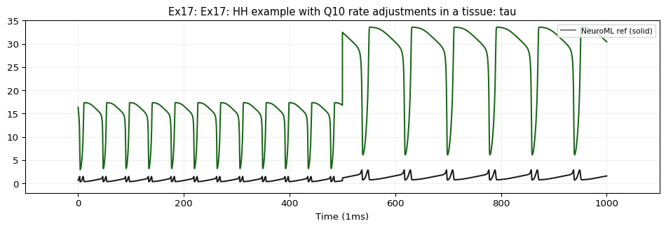
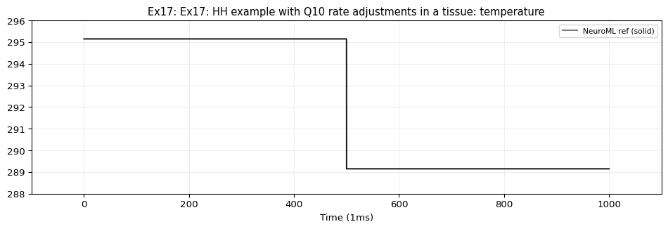
Demonstrates tissueWithVaryingTemperature — an HH cell with Q10-scaled gating rates inside a tissue that changes temperature from 22°C to 16°C at \(t=500\,\text{ms}\).

\[C\frac{dv}{dt} = -g_{Na}m^3h(v - E_{Na}) - g_K n^4(v - E_K) - g_L(v - E_L) + I_{\text{ext}}\]

Gate rates are scaled by \(Q_{10}(T)\): \[Q_{10}(T) = 3^{(T - 32)/10}\]

\(T = 22°C\) for \(t < 500\,\text{ms}\): \(Q_{10} = 3^{-1} = 1/3\)
\(T = 16°C\) for \(t \ge 500\,\text{ms}\): \(Q_{10} = 3^{-1.6} \approx 0.1724\)

1. Define in TVBO

from tvbo import SimulationExperiment

# Q10 temperature scaling: 3^((T-32)/10)
# T=22°C: Q10 = 3^(-1) = 0.333333
# T=16°C: Q10 = 3^(-1.6) = 0.172414
# Temperature changes at t=500ms (= 0.5s)
# Same HH conductances as Ex1/Ex5/Ex10: g_Na=1200nS, g_K=360nS, g_L=3nS, C=10pF
# Constant input: 0.08nA = 80pA for entire simulation

exp = SimulationExperiment.from_string("""
label: "NeuroML Ex17: HH Tissue with Q10"
dynamics:
  name: HH_Tissue_Q10
  parameters:
    C:     { value: 10.0 }
    g_Na:  { value: 1200.0 }
    g_K:   { value: 360.0 }
    g_L:   { value: 3.0 }
    E_Na:  { value: 50.0 }
    E_K:   { value: -77.0 }
    E_L:   { value: -54.3 }
    I_amp: { value: 0.08 }
    Q10_early: { value: 0.333333, description: "Q10 at 22C: 3^(-1)" }
    Q10_late:  { value: 0.172414, description: "Q10 at 16C: 3^(-1.6)" }
    switch_time: { value: 500.0, unit: ms, description: "Temperature switch at 500ms" }
  derived_variables:
    Q10:
      equation:
        rhs: "Piecewise((Q10_early, t < switch_time), (Q10_late, True))"
      description: "Q10 factor: switches from 22C to 16C at 500ms"
    I_ext:
      equation:
        rhs: "I_amp"
      description: "Constant current 0.08 nA"
    alpha_m:
      equation:
        rhs: "Piecewise((1.0, Eq(v, -40.0)), (0.1*(v + 40.0)/(1.0 - exp(-(v + 40.0)/10.0)), True))"
    beta_m:
      equation:
        rhs: "4.0*exp(-(v + 65.0)/18.0)"
    alpha_h:
      equation:
        rhs: "0.07*exp(-(v + 65.0)/20.0)"
    beta_h:
      equation:
        rhs: "1.0/(1.0 + exp(-(v + 35.0)/10.0))"
    alpha_n:
      equation:
        rhs: "Piecewise((0.1, Eq(v, -55.0)), (0.01*(v + 55.0)/(1.0 - exp(-(v + 55.0)/10.0)), True))"
    beta_n:
      equation:
        rhs: "0.125*exp(-(v + 65.0)/80.0)"
  state_variables:
    v:
      equation:
        rhs: "(-g_Na*m**3*h*(v - E_Na) - g_K*n**4*(v - E_K) - g_L*(v - E_L) + I_ext*1000) / C"
      initial_value: -65.0
      variable_of_interest: true
    m:
      equation: { rhs: "Q10*(alpha_m*(1 - m) - beta_m*m)" }
      initial_value: 0.052932
    h:
      equation: { rhs: "Q10*(alpha_h*(1 - h) - beta_h*h)" }
      initial_value: 0.596121
    n:
      equation: { rhs: "Q10*(alpha_n*(1 - n) - beta_n*n)" }
      initial_value: 0.317677
network:
  number_of_nodes: 1
integration:
  method: euler
  step_size: 0.01
  duration: 1000.0
  time_scale: ms
""")
print(f"Model: {exp.dynamics.name}")
print(f"SVs: {list(exp.dynamics.state_variables.keys())}")

Model: HH_Tissue_Q10
SVs: ['h', 'm', 'n', 'v']

2. Render LEMS XML

xml = exp.render("lems")
print(xml[:1200])


<Lems>

  <!-- Tell jLEMS/jNeuroML which component is the simulation entry point. -->
  <Target component="sim_NeuroML_Ex17__HH_Tissue_with_Q10"/>

  <!-- ════════════════════════════════════════════════════════════════
       Dimensions & Units (inline — no external includes needed)
       ════════════════════════════════════════════════════════════════ -->

  <!-- Dimensions -->
  <Dimension name="none"/>
  <Dimension name="time" t="1"/>
  <Dimension name="voltage" m="1" l="2" t="-3" i="-1"/>
  <Dimension name="per_time" t="-1"/>
  <Dimension name="conductance" m="-1" l="-2" t="3" i="2"/>
  <Dimension name="capacitance" m="-1" l="-2" t="4" i="2"/>
  <Dimension name="current" i="1"/>
  <Dimension name="resistance" m="1" l="2" t="-3" i="-2"/>
  <Dimension name="concentration" l="-3" n="1"/>
  <Dimension name="substance" n="1"/>
  <Dimension name="charge" t="1" i="1"/>
  <Dimension name="temperature" k="1"/>

  <!-- Units -->
  <Unit symbol="s" dimension="time" power="0"/>
  <Unit symbol="ms" dimension="time" power="-3"/>
  <Unit symbol="us" dimension="time" power="-6"/>
  <Unit symbol="V" dimension="voltage" power="0"/>
  <Unit symbol="mV" dimension="voltage" power="-3"/>
  <Unit

3. Run Reference

import sys, os
sys.path.insert(0, os.path.dirname(os.path.abspath(".")))
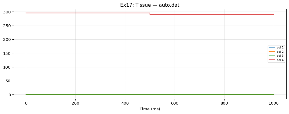
from _nml_helpers import run_lems_example

ref_outputs = run_lems_example("LEMS_NML2_Ex17_Tissue.xml")
for name, arr in ref_outputs.items():
    print(f"  {name}: shape={arr.shape}")

  auto.dat: shape=(100001, 5)

4. Run TVBO

import numpy as np

result = exp.run("neuroml")
da = result.integration.data
tvbo_arr = np.column_stack([da.coords['time'].values, da.values])
print(f"TVBO: shape={tvbo_arr.shape}")

TVBO: shape=(100001, 5)

5. Plot Reference

import matplotlib.pyplot as plt
import numpy as np

for name, ref_arr in ref_outputs.items():
    t = ref_arr[:, 0] * 1000
    fig, ax = plt.subplots(figsize=(10, 4))
    for i in range(1, min(ref_arr.shape[1], 6)):
        ax.plot(t, ref_arr[:, i], alpha=0.8, label=f'col {i}')
    ax.set_xlabel("Time (ms)")
    ax.set_title(f"Ex17: Tissue — {name}")
    ax.legend(fontsize=7)
    ax.grid(True, alpha=0.3)
    plt.tight_layout()
    plt.show()

Continuous Projections

continuousProjection and continuousConnection are NeuroML-native network features for graded synaptic transmission. TVBO represents the FHN cell dynamics; the continuous coupling is handled by the NeuroML adapter.