Defining Networks

How to create, visualize, save, and load brain network connectivity

A Network describes the connectivity structure between brain regions: nodes (regions) connected by weighted edges (tracts). TVBO provides several ways to create networks — from inline YAML, from matrices, from files, or from the tvbo platform.

from tvbo import Network

1. From YAML Strings

The simplest way to define a small network. Each node has an id and label; each edge connects a source to a target with optional parameters.

net = Network.from_string("""
label: Visual Pathway

nodes:
  - {id: 0, label: V1}
  - {id: 1, label: V2}
  - {id: 2, label: MT}

edges:
  - source: 0
    target: 1
    parameters:
      weight:
        value: 0.7
      distance:
        value: 25
        unit: mm
  - source: 1
    target: 2
    parameters:
      weight:
        value: 0.4
      distance:
        value: 40
        unit: mm
  - source: 0
    target: 2
    parameters:
      weight:
        value: 0.2
      distance:
        value: 60
        unit: mm
""")

net.plot_graph()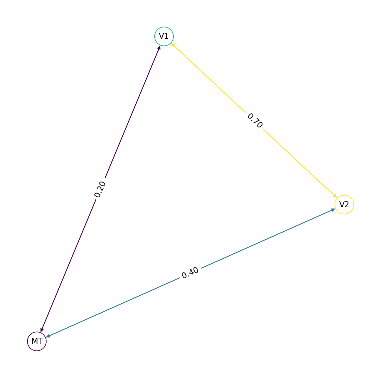

Edges are undirected by default — the connection goes both ways. Set directed: true for one-way connections:

net_dir = Network.from_string("""
label: Feedforward Chain

nodes:
  - {id: 0, label: V1}
  - {id: 1, label: V2}
  - {id: 2, label: MT}

edges:
  - source: 0
    target: 1
    directed: true
    parameters:
      weight: {value: 0.7}
  - source: 1
    target: 2
    directed: true
    parameters:
      weight: {value: 0.4}
""")

net_dir.plot_graph()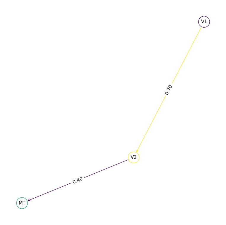

2. From Matrices

For larger networks, pass NumPy weight and length matrices directly:

import numpy as np

W = np.array([
    [0.0, 0.5, 0.3, 0.0],
    [0.5, 0.0, 0.8, 0.2],
    [0.3, 0.8, 0.0, 0.6],
    [0.0, 0.2, 0.6, 0.0],
])

L = np.array([
    [0,  50, 80,  0],
    [50,  0, 30, 70],
    [80, 30,  0, 40],
    [0,  70, 40,  0],
])

net = Network.from_matrix(W, lengths=L, labels=["V1", "V2", "MT", "PFC"])
net.plot_overview()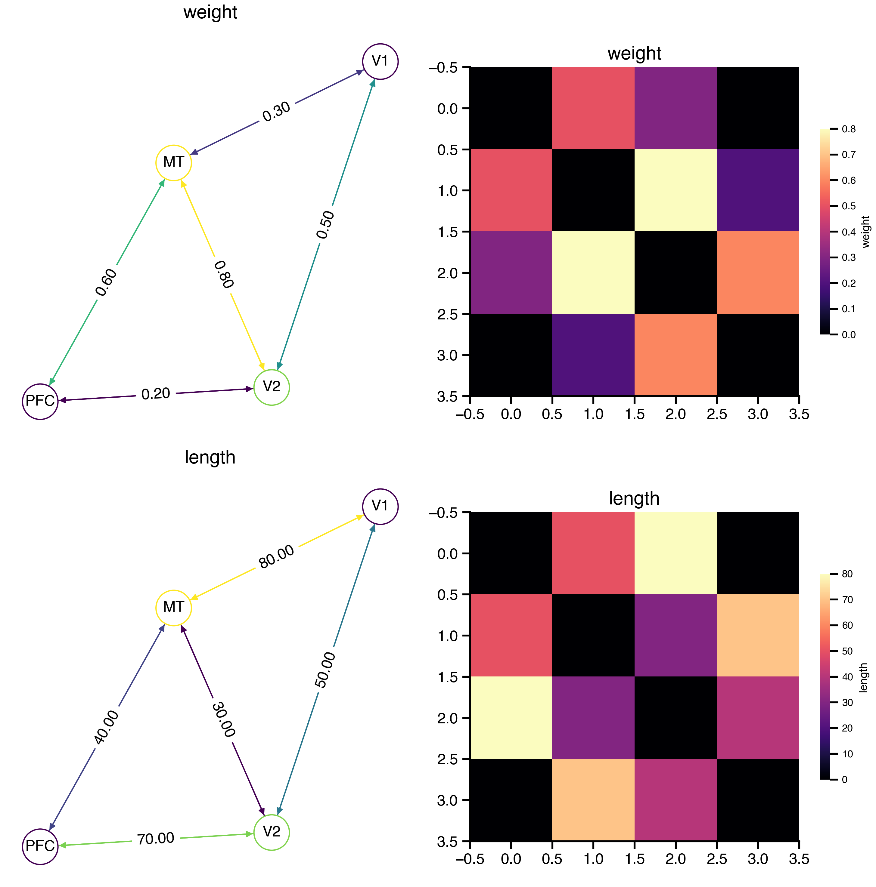

The weight and length matrices are accessible as properties:

print(f"{net.number_of_nodes} nodes")
print(f"Weights range: [{net.weights_matrix.min():.1f}, {net.weights_matrix.max():.1f}]")
print(f"Mean length:   {net.lengths_matrix.mean():.0f} mm")

4 nodes
Weights range: [0.0, 0.8]
Mean length:   34 mm

3. Saving and Loading

Networks are stored as a YAML sidecar (metadata) paired with an HDF5 companion file (matrix data). This keeps metadata readable while storing large matrices efficiently.

Save

import tempfile
from pathlib import Path

tmpdir = Path(tempfile.mkdtemp())

net.save(tmpdir / "visual.yaml")
print("Created files:")
for f in sorted(tmpdir.iterdir()):
    sz = f.stat().st_size
    print(f"  {f.name:20s}  ({sz:,} bytes)")

Created files:
  visual.h5             (17,136 bytes)
  visual.yaml           (532 bytes)

The sidecar is plain YAML — human-readable and schema-valid:

print((tmpdir / "visual.yaml").read_text())

tvbo_class: tvbo:Network
schema_version: tvb-datamodel/0.7.0
number_of_nodes: 4
distance_unit: mm
time_unit: ms
data_file: visual.h5
parameters:
  conduction_speed:
    label: v
    value: 3.0
    unit: mm_per_ms
nodes:
- id: 0
  label: V1
- id: 1
  label: V2
- id: 2
  label: MT
- id: 3
  label: PFC
edges:
- label: weight
  format: dense
  weighted: true
  valid_diagonal: false
  non_negative: true
  directed: false
- label: length
  format: dense
  weighted: true
  valid_diagonal: false
  non_negative: true
  directed: false

Load

Loading is lazy: metadata is read immediately, but matrix data is only loaded from the HDF5 file on first access.

loaded = Network.from_file(tmpdir / "visual.yaml")

# Metadata — instant, no HDF5 I/O
print(f"Nodes: {loaded.number_of_nodes}")

# Arrays — loaded on first access
print(f"Weights shape: {loaded.weights_matrix.shape}")
np.testing.assert_allclose(loaded.weights_matrix, W)
print("Roundtrip OK ✓")

Nodes: 4
Weights shape: (4, 4)
Roundtrip OK ✓

4. Data Format

The save() call produces two files:

File	Content	Format
YAML sidecar	Nodes, labels, schema fields	Human-readable text
HDF5 companion	Weight/length matrices	Compressed binary

This sidecar + companion pattern keeps metadata inspectable while storing large matrices efficiently.

HDF5 Structure

The companion file organizes matrices under an edges/ hierarchy:

Inspect HDF5 companion structure

import h5py

with h5py.File(tmpdir / "visual.h5", "r") as f:
    print(f"Root attributes:")
    for k, v in f.attrs.items():
        print(f"  {k}: {v}")
    print()
    def show(name, obj):
        if isinstance(obj, h5py.Dataset):
            print(f"  {name:40s}  shape={obj.shape}  dtype={obj.dtype}")
        elif isinstance(obj, h5py.Group):
            attrs = {k: str(v) for k, v in obj.attrs.items()}
            if attrs:
                print(f"  {name:40s}  {attrs}")
    f.visititems(show)

Root attributes:
  schema_version: tvb-datamodel/0.7.0
  sidecar_file: visual.yaml
  tvbo_class: tvbo:Network

  edges/length                              {'directed': 'False', 'format': 'dense', 'shape': '[4 4]', 'tvbo_class': 'tvbo:Matrix'}
  edges/length/data                         shape=(4, 4)  dtype=float32
  edges/weight                              {'directed': 'False', 'format': 'dense', 'shape': '[4 4]', 'tvbo_class': 'tvbo:Matrix'}
  edges/weight/data                         shape=(4, 4)  dtype=float32

Each edge group (edges/weights, edges/lengths) stores:

format attr — "dense", "csr", or "coo"
shape attr — matrix dimensions \([N, N]\)
data dataset — matrix values (dense) or nonzero values (sparse)
For CSR: additional indices + indptr datasets
For COO: additional row + col datasets

Auto-Format Selection

Storage format is chosen automatically from matrix properties:

Condition	Format	Rationale
\(N < 500\) or fill \(> 30\%\)	Dense + gzip	Compression beats sparse indexing
\(N \geq 500\) and fill \(\leq 30\%\)	CSR	Sparse indexing wins at scale

Supported Backends

Backend	Extension	Use case
HDF5	`.h5`	Default — best compression, random access
Zarr	`.zarr/`	Cloud-native storage (S3, GCS)
CSV	`.csv`	Legacy, single matrix only

net.save("out.yaml", binary_format="zarr")    # Zarr companion
net.save("out.yaml", binary_format="csv")     # CSV, first matrix only
net.save("out.yaml", sidecar_format="json")   # JSON sidecar + HDF5

5. Built-in Connectomes

TVBO ships with normative connectomes from published tractography datasets. Load them by atlas name:

sc = Network.from_db("DesikanKilliany")
print(f"{sc.number_of_nodes} regions, atlas: {sc.atlas.name}")

87 regions, atlas: DesikanKilliany

sc.plot_overview(log_weights=True)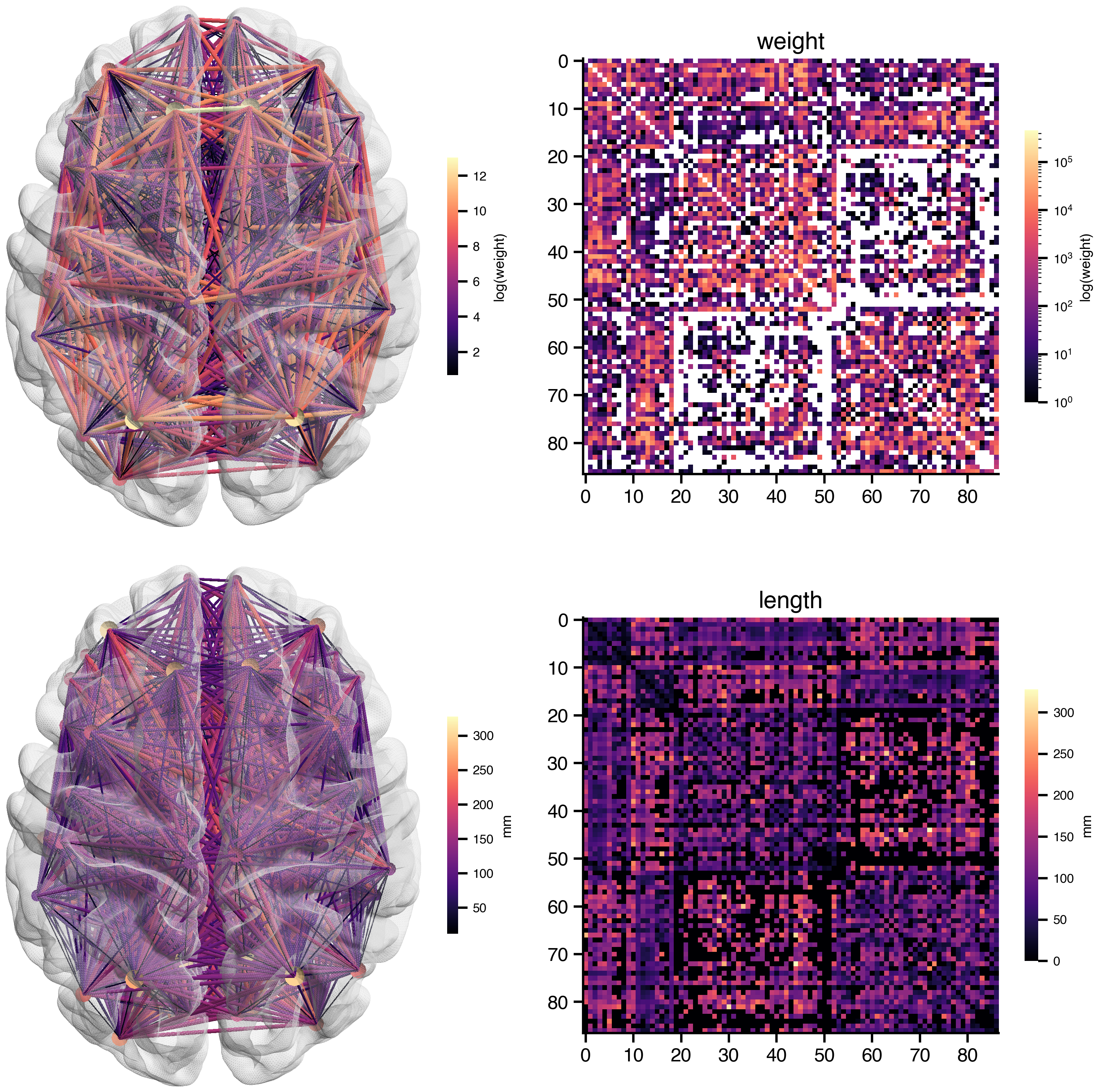

BIDS-Compliant File Naming

Network files in tvbo/database/networks/ follow the BEP017 naming convention:

tpl-<space>[_cohort-<source>]_rec-<pipeline>_atlas-<atlas>[_seg-<variant>][_scale-<N>]_desc-<modality>_relmat.<ext>

Entity	Meaning	Example
`tpl-`	Template/coordinate space	`MNI152NLin2009cAsym`
`cohort-`	Population cohort	`HCPYA`, `MghUscHcp32`, `PPMI85`
`rec-`	Reconstruction pipeline	`dTOR`, `MghUscHcp32`
`atlas-`	Brain parcellation	`DesikanKilliany`, `Schaefer2018`
`seg-`	Segmentation variant	`ranked`, `ordered`, `17Networks`
`scale-`	Number of parcels	`1000`
`desc-`	Descriptor	`SC` (structural connectivity)
`_relmat`	BEP017 suffix	Relationship matrix

Access the BIDS filename programmatically:

print(sc.bids_filename)

tpl-MNI152NLin2009cAsym_cohort-HCPYA_rec-dTOR_atlas-DesikanKilliany_desc-SC_relmat.h5

Transforms

Raw streamline counts vary over orders of magnitude. Apply min–max normalization to scale weights to \([0, 1]\):

print(
    f"Before transform: [{sc.weights_matrix.min():.2f}, {sc.weights_matrix.max():.2f}]"
)

sc.normalize()

print(
    f"After transform: [{sc.weights_matrix.min():.2f}, {sc.weights_matrix.max():.2f}]"
)

Before transform: [0.00, 458885.00]
After transform: [0.00, 1.00]

normalize() does not overwrite the stored matrix. Instead it appends a Function transform to the Network’s transforms list — the transformation is applied lazily when accessing weights_matrix. Multiple transforms on the same target are applied in order. Because the transforms are written into the YAML sidecar, every processing step is recorded for reproducibility:

# The YAML sidecar now contains the transforms
import yaml

meta = yaml.safe_load(sc.to_yaml())
print(yaml.dump({"transforms": meta.get("transforms")}, default_flow_style=False))

transforms:
- equation:
    latex: false
    rhs: (M - M_min) / (M_max - M_min)
  name: weight

The rhs field captures what was done, not just the result. Anyone who loads this YAML gets the same transformed weights — no hidden in-memory mutations, and the raw matrix in HDF5 stays untouched.

6. Delays from Tract Lengths

Transmission delays are computed from the lengths matrix and conduction speed (\(v\), default 3 mm/ms):

delays = sc.compute_delays()
print(f"Delay range: [{delays.min():.1f}, {delays.max():.1f}] ms")

Delay range: [0.0, 0.0] ms

7. Advanced: Multi-Layer Networks

The Network schema supports heterogeneous node dynamics, edge-level models, and variable routing — the building blocks for surface-based and multi-scale simulations.

7.1. Surface-Based Simulations

In surface-based simulations every vertex of the cortical mesh is a node. The simulation runs dynamics at vertex resolution — each of the ~10 000–160 000 vertices executes its own copy of the neural mass model. Two coupling mechanisms operate at different spatial scales:

Mechanism	Scale	Matrix	Delays
Local connectivity	vertex ↔︎ vertex	Sparse, based on geodesic distance kernel	instantaneous
Long-range SC	region ↔︎ region	Dense, from tractography	proportional to tract length

A region mapping (= node_mapping) array bridges the two scales: vertex states are averaged into region states for SC computation, and regional coupling is broadcast back to vertices.

TVBO representation

TVBO uses hierarchical network composition to represent both scales in one consistent structure:

Parent Network — region-level SC (\(N_\text{regions}\) nodes, weight and tract-length matrices).
Child Network — vertex-level local connectivity (\(N_\text{vertices}\) nodes, sparse LC matrix).
- parent_network → path to the parent SC file.
- node_mapping → HDF5 dataset /nodes/parent_index, the \(\text{int32}(N_\text{vertices},)\) region-mapping array.

Parent Network (dk_sc.yaml + dk_sc.h5)
├── 87 DK region nodes
├── edges/weights/data    (87 × 87)   dense
└── edges/lengths/data    (87 × 87)   dense

Child Network (surface_rh.yaml + surface_rh.h5)
├── parent_network: dk_sc.yaml
├── 2 562 vertex nodes  (fsaverage 3k, RH)
├── edges/weights/       CSR sparse  (2 562 × 2 562, fill ~10 %)
│   ├── data      (nnz,)
│   ├── indices   (nnz,)
│   └── indptr    (2 563,)
└── nodes/parent_index   int32 (2 562,)   ← region_mapping

Loading the surface and parcellation

The fsaverage pial surface and the Desikan–Killiany parcellation labels are fetched from templateflow. The parcellation labels are the region_mapping — each integer assigns a vertex to a DK region:

Load surface mesh and parcellation from templateflow

from templateflow import api as tflow
import nibabel as nib
from bsplot.data.surface import get_surface_geometry
import numpy as np

# --- Surface mesh (3k ≈ 2 562 vertices per hemisphere) ---
vertices_rh, faces_rh = get_surface_geometry(
    template="fsaverage", hemi="rh", density="3k", suffix="pial",
)
n_vertices = vertices_rh.shape[0]

# --- Parcellation labels = region_mapping ---
gii = nib.load(
    tflow.get("fsaverage", hemi="R", density="3k",
              atlas="Desikan2006", suffix="dseg", extension=".label.gii")
)
region_mapping = gii.darrays[0].data.astype(np.int32)
label_names = gii.labeltable.get_labels_as_dict()
n_regions = len([k for k in label_names if k != 0])

print(f"Surface: {n_vertices:,} vertices (nodes)")
print(f"Parcellation: {n_regions} cortical regions")
print(f"region_mapping: int32({n_vertices},) — maps every vertex to its DK region")
print(f"  e.g. vertex 0 → region {region_mapping[0]} ({label_names[region_mapping[0]]})")

Surface: 2,562 vertices (nodes)
Parcellation: 35 cortical regions
region_mapping: int32(2562,) — maps every vertex to its DK region
  e.g. vertex 0 → region 24 (precentral)

Building the local connectivity

Local connectivity encodes lateral cortical coupling — a sparse kernel based on geodesic distance along the surface mesh (typically Gaussian with \(\sigma \approx 10\,\)mm, truncated at 30–40 mm). Here we approximate with Euclidean distance for demonstration:

Build sparse local connectivity matrix (Gaussian kernel)

from scipy.spatial import cKDTree
from scipy.sparse import coo_matrix

cutoff_mm = 30.0   # only connect vertices within 30 mm
sigma_mm = 10.0    # Gaussian kernel width

tree = cKDTree(vertices_rh)
pairs = np.array(list(tree.query_pairs(r=cutoff_mm)))  # (n_pairs, 2)
dists = np.linalg.norm(
    vertices_rh[pairs[:, 0]] - vertices_rh[pairs[:, 1]], axis=1,
)
weights = np.exp(-dists**2 / (2 * sigma_mm**2))

# Build symmetric sparse matrix (COO → CSR)
rows = np.concatenate([pairs[:, 0], pairs[:, 1]])
cols = np.concatenate([pairs[:, 1], pairs[:, 0]])
data = np.concatenate([weights, weights])
LC = coo_matrix((data, (rows, cols)), shape=(n_vertices, n_vertices)).tocsr()

fill = LC.nnz / n_vertices**2
print(f"Local connectivity: {n_vertices} × {n_vertices}, "
      f"nnz = {LC.nnz:,}, fill = {fill:.1%}")
print(f"Storage: {(LC.nnz * 12 + (n_vertices + 1) * 4) / 1024:.0f} KB (CSR)")

Local connectivity: 2562 × 2562, nnz = 622,610, fill = 9.5%
Storage: 7306 KB (CSR)

Creating the hierarchical Network

The region-level SC is the parent. The vertex-level LC is the child, linked via parent_network and node_mapping:

# --- Parent: region-level SC ---
sc = Network.from_db("DesikanKilliany")
sc.save(tmpdir / "dk_sc.yaml")

# --- Child: vertex-level local connectivity ---
surface_net = Network.from_matrix(LC.toarray())
surface_net.label = "fsaverage 3k Surface Network (RH)"

# Link child → parent and attach the region mapping.
# parent_network accepts a Network object — the filepath
# reference is derived automatically from the parent's save path.
surface_net.set_node_mapping(region_mapping, parent_network=sc)

# Save — node_mapping is written to HDF5 automatically
surface_net.save(tmpdir / "surface_rh.yaml")

print("Parent SC:")
print(f"  {sc.number_of_nodes} region nodes")
print(f"Child surface Network:")
print(f"  {surface_net.number_of_nodes} vertex nodes")
print(f"  parent_network: {surface_net.parent_network}")
print(f"  node_mapping:   {surface_net.node_mapping}")

Parent SC:
  87 region nodes
Child surface Network:
  2562 vertex nodes
  parent_network: dk_sc.yaml
  node_mapping:   /nodes/parent_index

HDF5 companion structure

The parent stores dense SC matrices; the child stores the sparse LC matrix and the parent_index region-mapping array:

Inspect HDF5 companion structure

for name in ["dk_sc.h5", "surface_rh.h5"]:
    path = tmpdir / name
    print(f"\n--- {name} ({path.stat().st_size / 1024:.0f} KB) ---")
    with h5py.File(path, "r") as hf:
        def _show(dset_name, obj):
            if isinstance(obj, h5py.Dataset):
                print(f"  {dset_name:40s}  {obj.shape}  {obj.dtype}")
            elif isinstance(obj, h5py.Group):
                for k, v in obj.attrs.items():
                    print(f"  {dset_name:40s}  [{k}={v}]")
        hf.visititems(_show)


--- dk_sc.h5 (77 KB) ---
  edges/length                              [directed=False]
  edges/length                              [format=dense]
  edges/length                              [shape=[87 87]]
  edges/length                              [tvbo_class=tvbo:Matrix]
  edges/length                              [unit=mm]
  edges/length/data                         (87, 87)  float32
  edges/weight                              [directed=False]
  edges/weight                              [format=dense]
  edges/weight                              [shape=[87 87]]
  edges/weight                              [tvbo_class=tvbo:Matrix]
  edges/weight/data                         (87, 87)  float32
  nodes/coordinates                         (87, 3)  float32

--- surface_rh.h5 (4894 KB) ---
  edges/weight                              [directed=False]
  edges/weight                              [format=csr]
  edges/weight                              [shape=[2562 2562]]
  edges/weight                              [tvbo_class=tvbo:Matrix]
  edges/weight/data                         (622610,)  float32
  edges/weight/indices                      (622610,)  int32
  edges/weight/indptr                       (2563,)  int32
  nodes/parent_index                        (2562,)  int32

Visualizing the two-scale structure

The parcellation colours show which vertices belong to each region (= one row/column of the parent SC matrix). The network overlay shows the long-range structural connections between regions:

Visualize parcellation + SC network on cortical surface

import matplotlib.pyplot as plt
from bsplot.surface import plot_surf
from bsplot.graph import (
    get_centers_from_surface_parc, create_network,
    create_node_mesh, create_edge_mesh,
)

# --- Use 10k surface for sharper rendering ---
verts_10k, _ = get_surface_geometry(
    template="fsaverage", hemi="rh", density="10k", suffix="pial",
)
labels_10k = nib.load(
    tflow.get("fsaverage", hemi="R", density="10k",
              atlas="Desikan2006", suffix="dseg", extension=".label.gii")
).darrays[0].data

# Region centroids on the surface (for node placement)
centers = get_centers_from_surface_parc(verts_10k, labels_10k)

# Build a NetworkX graph from the SC matrix (RH cortical regions only)
sc.normalize()
W = sc.weights_matrix
rh_ids = sorted(k for k in centers.keys() if k != 0)
n_rh = len(rh_ids)
rh_centers = {i: centers[rh_ids[i]] for i in range(n_rh)}
W_rh = np.zeros((n_rh, n_rh))
for i, ri in enumerate(rh_ids):
    for j, rj in enumerate(rh_ids):
        if ri < W.shape[0] and rj < W.shape[0]:
            W_rh[i, j] = W[ri, rj]

G = create_network(rh_centers, W_rh, threshold_percentile=90)

# Assign each node its DK region label (for colour matching)
for i, rid in enumerate(rh_ids):
    if i in G:
        G.nodes[i]["region_id"] = float(rid)

# Node mesh coloured by region ID (same colormap as the surface)
cmap = plt.cm.tab20
max_label = float(max(rh_ids))
node_mesh, node_overlay = create_node_mesh(
    G, radius=1.8, resolution=16, data_key="region_id",
)
edge_mesh = create_edge_mesh(G, radius=0.08, resolution=8)

# --- Plot: parcellated surface + colour-matched SC network ---
fig, ax = plt.subplots(figsize=(5, 5))
plot_surf(
    "fsaverage",
    hemi="rh",
    view="lateral",
    ax=ax,
    surface_density="10k",
    surface_suffix="pial",
    alpha=0.3,
    overlay=labels_10k.astype(float),
    cmap="tab20",
    parcellated=True,
    additional_surfaces=[node_mesh, edge_mesh],
    additional_overlays=[node_overlay, None],
    additional_cmaps=["tab20", None],
    additional_vmins=[0.0, None],
    additional_vmaxs=[max_label, None],
    additional_colors=[None, "steelblue"],
    additional_alphas=[1.0, 0.6],
)
ax.set_title("Surface simulation: parcellation + SC network", fontsize=10)
ax.axis("off")
plt.show()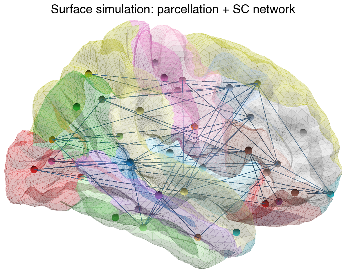

Each coloured surface patch is the territory of one region node. All vertices within a patch share the same long-range SC input (broadcast via region_mapping), while local connectivity couples each vertex to its cortical neighbours.

7.2 Multi-Scale Co-Simulation

Multi-scale brain simulations couple a macroscale mean-field network with a microscale spiking subnetwork. A selected region node acts as a proxy — its mean-field dynamics are replaced by the aggregate activity of a detailed spiking population. The remaining network stays mean-field, exchanging firing rates and coupling currents with the spiking subnetwork through interface edges.

TVBO represents this in a single YAML + HDF5 file pair using hierarchical network composition: macroscale (mean-field) and microscale (spiking) nodes coexist in one network, linked by node_mapping. The proxy node’s state is driven by the aggregate output of its child subnetwork.

Architecture

The proxy pattern used here is compatible with tvb-multiscale’s co-simulation architecture, where:

Proxy nodes in the mean-field network are not simulated locally — their state is replaced by spiking network output
Input proxies (TVB → spiking) inject mean-field activity as stimulation into the spiking population
Output proxies (spiking → TVB) record aggregate spiking activity and transform it back to mean-field state variables
Transformers handle scale translation (e.g., spike trains → instantaneous firing rate → synaptic gating variable \(S\))

graph TD
    subgraph NET["<b>multiscale_cortex.yaml + .h5</b>"]
        V1["<b>Node 0 — V1</b><br/><i>ReducedWongWang</i>"]
        V2["<b>Node 1 — V2 (proxy)</b><br/><i>ReducedWongWang</i><br/>state ↔ subnetwork aggregate"]

        V1 -- "S → c_pop &ensp; w = 0.5" --> V2
        V2 -- "S → c_pop &ensp; w = 0.3" --> V1

        subgraph SUB["Spiking subnetwork &ensp;·&ensp; node_mapping: all → 1"]
            direction LR
            E["E₁ – E₂ – E₃ – … – E₈<br/><i>Izhikevich</i>"]
            I["I₁ – I₂<br/><i>Izhikevich</i>"]
            E <-- "10×10 weight matrix in HDF5" --> I
        end

        V2 -- "source_var: S → target_var: I<br/><i>I = gain · S · N_E</i>" --> SUB
    end

    style NET fill:#99999900,stroke:#333,stroke-width:2px
    style SUB fill:#e8f4fd,stroke:#4a90d9,stroke-width:1px,stroke-dasharray:5
    style V1 fill:#fff,stroke:#333
    style V2 fill:#fff3cd,stroke:#856404
    style E fill:#d4edda,stroke:#155724
    style I fill:#f8d7da,stroke:#721c24

Figure 1: Multi-scale co-simulation architecture

Network Definition

The entire multi-scale setup lives in a single YAML file. YAML anchors (&) and aliases (*) eliminate redundancy — dynamics and coupling are defined once and referenced everywhere:

Node 0 is a regular mean-field region (ReducedWongWang)
Node 1 is a proxy — during co-simulation its mean-field state is replaced by the aggregate output of the child subnetwork (10 Izhikevich spiking neurons)
parent_network on the child points back to this file; node_mapping maps all 10 spiking neurons to parent node 1

from IPython.display import Markdown
from pathlib import Path

ms_yaml_path = Path("multiscale_cortex.yaml")
ms_yaml = ms_yaml_path.read_text()
Markdown(f"```yaml\n{ms_yaml}```")

# multiscale_cortex.yaml — hybrid mean-field / spiking network
label: Multi-Scale Cortex

# ── Dynamics (defined once, referenced by anchor) ───────────
dynamics:
  ReducedWongWang: &rww
    name: ReducedWongWang
  Izhikevich: &izh
    name: Izhikevich
    state_variables:
      v:
        equation:
          rhs: "0.04*v*v + 5*v + 140 - u + I"
      u:
        equation:
          rhs: "a * (b*v - u)"
    parameters:
      a: {value: 0.02}
      b: {value: 0.2}
      c: {value: -65}
      d: {value: 8}

# ── Coupling (defined once, referenced by anchor) ──────────
coupling:
  linear: &linear
    name: linear
  excitatory: &exc
    name: excitatory
  inhibitory: &inh
    name: inhibitory

# ── Macroscale nodes ────────────────────────────────────────
nodes:
  # Mean-field regions
  - {id: 0, label: V1, dynamics: *rww}
  - {id: 1, label: V2 (proxy), dynamics: *rww}
  # Spiking subnetwork (children of node 1)
  - {id: 2,  label: E1, dynamics: *izh}
  - {id: 3,  label: E2, dynamics: *izh}
  - {id: 4,  label: E3, dynamics: *izh}
  - {id: 5,  label: E4, dynamics: *izh}
  - {id: 6,  label: E5, dynamics: *izh}
  - {id: 7,  label: E6, dynamics: *izh}
  - {id: 8,  label: E7, dynamics: *izh}
  - {id: 9,  label: E8, dynamics: *izh}
  - {id: 10, label: I1, dynamics: *izh,
     state: [{name: v, value: -65}, {name: u, value: -14}]}
  - {id: 11, label: I2, dynamics: *izh,
     state: [{name: v, value: -65}, {name: u, value: -14}]}

# ── Node mapping: spiking neuron → parent proxy node ───────
# int32 array of length 12: [–1, –1, 1, 1, 1, 1, 1, 1, 1, 1, 1, 1]
#   –1 = top-level node (no parent)
#    1 = child of node 1 (the proxy)
node_mapping: /nodes/parent_index

# ── Edges ───────────────────────────────────────────────────
edges:
  # ── Macroscale edges (mean-field ↔ proxy) ──
  - source: 0
    target: 1
    directed: true
    source_var: S            # synaptic gating output
    target_var: c_pop        # population coupling input
    parameters:
      weight: {value: 0.5}
    coupling: *linear
  - source: 1
    target: 0
    directed: true
    source_var: S
    target_var: c_pop
    parameters:
      weight: {value: 0.3}
    coupling: *linear

  # ── Subnetwork template edge (10×10 local connectivity) ──
  - label: weights
    format: dense
    weighted: true
    directed: true
    valid_diagonal: false
    non_negative: true

  # ── Explicit E↔I edges within subnetwork ──
  - {source: 2, target: 10, directed: true,
     parameters: {weight: {value: 0.5}}, coupling: *exc}
  - {source: 10, target: 2, directed: true,
     parameters: {weight: {value: -0.3}}, coupling: *inh}

  # ── Interface edges (proxy ↔ subnetwork) ──
  - source: 1                 # proxy node (mean-field)
    target: 2                 # first excitatory neuron
    directed: true
    source_var: S              # mean-field gating → spiking current
    target_var: I
    parameters:
      weight: {value: 1.0}
      gain: {value: 0.1}      # transformer scaling: I = gain · S · N_E
    coupling: *linear

Saving and Loading

The only custom code is the random subnetwork connectivity. Everything else — YAML sidecar, HDF5 companion, matrix storage format — is handled automatically by Network:

Generate random sparse subnetwork connectivity (8E + 2I)

N_sub = 10   # spiking subnetwork size (8E + 2I)

# Random sparse local connectivity (E→E, E→I, I→E)
rng = np.random.default_rng(42)
W_sub = np.zeros((N_sub, N_sub))
# E→E: sparse random (p=0.3)
for i in range(8):
    for j in range(8):
        if i != j and rng.random() < 0.3:
            W_sub[i, j] = rng.uniform(0.1, 0.5)
# E→I
for i in range(8):
    for j in range(8, 10):
        if rng.random() < 0.5:
            W_sub[i, j] = rng.uniform(0.2, 0.6)
# I→E (inhibitory)
for i in range(8, 10):
    for j in range(8):
        if rng.random() < 0.4:
            W_sub[i, j] = rng.uniform(0.1, 0.4)

print(f"Subnetwork: {N_sub}×{N_sub}, "
      f"fill: {np.count_nonzero(W_sub) / W_sub.size:.0%}")

Subnetwork: 10×10, fill: 29%

Create the network from the YAML file and attach the matrix:

net = Network.from_string(ms_yaml)
print(f"Nodes:          {len(net.nodes)}")
print(f"Template edges: {sum(1 for e in net.edges if getattr(e, 'source', None) is None)}")
print(f"Explicit edges: {sum(1 for e in net.edges if getattr(e, 'source', None) is not None)}")

Nodes:          12
Template edges: 1
Explicit edges: 5

Attach the subnetwork weight matrix and save — Network.save() writes the YAML sidecar and HDF5 companion automatically:

# Attach matrix (matches template edge label: weights)
# Embed the 10×10 subnetwork into the full 12×12 node space
# Nodes 0–1 are mean-field; nodes 2–11 are the spiking subnetwork
W_full = np.zeros((12, 12))
W_full[2:, 2:] = W_sub
net._cached_weights = W_full

# Save → creates .yaml sidecar + .h5 companion
net.save(tmpdir / "multiscale_cortex.yaml")

for f in sorted(tmpdir.glob("multiscale*")):
    print(f"  {f.name:30s}  ({f.stat().st_size:,} bytes)")

  multiscale_cortex.h5            (11,400 bytes)
  multiscale_cortex.yaml          (6,111 bytes)

Roundtrip — load the saved network and verify the matrix:

loaded = Network.from_file(tmpdir / "multiscale_cortex.yaml")

# Metadata — instant (no HDF5 I/O)
print(f"Nodes: {len(loaded.nodes)}")
print(f"Edges: {len(loaded.edges)}")
print(f"Node mapping: {loaded.node_mapping}")

# Matrix — lazy-loaded on first access
np.testing.assert_allclose(loaded.weights_matrix, W_full)
print(f"Matrix shape: {loaded.weights_matrix.shape}")
print(f"Roundtrip OK ✓")

Nodes: 12
Edges: 6
Node mapping: /nodes/parent_index
Matrix shape: (12, 12)
Roundtrip OK ✓

Inspect the HDF5 companion structure:

Inspect HDF5 companion structure

import h5py

with h5py.File(tmpdir / "multiscale_cortex.h5", "r") as f:
    def show(name, obj):
        if isinstance(obj, h5py.Dataset):
            print(f"  {name:40s}  shape={obj.shape}  dtype={obj.dtype}")
        elif isinstance(obj, h5py.Group):
            attrs = {k: str(v) for k, v in obj.attrs.items()}
            if attrs:
                print(f"  {name:40s}  {attrs}")
    f.visititems(show)

  edges/weights                             {'directed': 'True', 'format': 'dense', 'shape': '[12 12]', 'tvbo_class': 'tvbo:Matrix'}
  edges/weights/data                        shape=(12, 12)  dtype=float32

The template edge label: weights tells save() to write the matrix at edges/weights/data in HDF5. On load, the same label routes the lazy reader back to the right dataset. No manual h5py code needed — the Network API handles the full sidecar + companion lifecycle.

Interface Variables

The interface edges between the proxy (node 1) and the subnetwork route specific state variables across scales. This is where the transformer logic lives — converting between mean-field and spiking representations:

Direction	Source Variable	Target Variable	Transformation
TVB → spiking	`S` (synaptic gating)	`I` (input current)	\(I = g \cdot S \cdot N_E\)
Spiking → TVB	spike trains	`S`, `R` (gating, rate)	\(\frac{dS}{dt} = -\frac{S}{\tau_s} + (1-S) R \gamma\)

The transformer converts spike trains to instantaneous firing rates (via kernel convolution or binning), then integrates the mean-field synaptic ODE to produce \(S\) and \(R\) values compatible with the parent network’s state space.

Schema Features for Multi-Scale

Feature	Schema Field	Purpose
Node-level models	`nodes[].dynamics`	Different ODE per region
Proxy identification	`node_mapping[i] >= 0`	Region replaced by spiking detail
Hierarchical nesting	`node_mapping`	Maps child nodes → parent proxy node
Variable routing	`source_var`, `target_var`	Connect specific state variables across scales
Per-edge coupling	`edges[].coupling`	Different coupling per connection
Per-node state	`nodes[].state`	Initial conditions per neuron
YAML anchors	`&rww`, `rww`, `&izh`, `izh`	Define once, reuse everywhere

Framework Interoperability

The single-file network representation maps naturally to multiple simulation backends:

Framework	Mean-Field Nodes	Spiking Subnetwork	Interface
tvb-multiscale	TVB `CoSimulator` with `proxy_inds=[1]`	NEST/ANNarchy `SpikingNetwork`	Proxy devices + transformers
JAX / tvb-optim	Vectorized mean-field ODE	Vectorized Izhikevich ODE (10 neurons)	Differentiable rate↔︎spike transform
NeuroML	`<population>` of rate neurons	`<population>` of `<izhikevichCell>`	`<continuousProjection>` for rate coupling
NetworkDynamics.jl	`ODEVertex` per mean-field node	`ODEVertex` per spiking neuron	`StaticEdge` or `ODEEdge` with routing

Each backend adapter reads the same YAML + HDF5 pair and generates backend-specific code:

tvb-multiscale: node_mapping identifies proxy nodes, source_var/target_var on interface edges configure VOI mappings and transformer selection
JAX: generates a combined ODE system where the subnetwork neurons are additional state dimensions, coupled via differentiable transformers
NeuroML: exports <population> elements per dynamics type with <continuousProjection> connections routing the declared variables between populations

Edge Dynamics

Edges can carry their own state variables — useful for synaptic plasticity or adaptation:

edges:
  - source: 0
    target: 1
    dynamics:
      name: STDP
      state_variables:
        w:
          equation:
            rhs: "A_plus * pre * post - A_minus * pre * post"
      parameters:
        A_plus:
          value: 0.01
        A_minus:
          value: 0.012

Here the edge weight \(w\) evolves according to its own ODE during simulation, implementing spike-timing-dependent plasticity.

7.3 Forward Model (Sensor Projection)

A forward model maps region-level brain activity to sensor-level recordings (EEG, MEG, iEEG). The projection is stored as a gain matrix \(G \in \mathbb{R}^{N_\text{sensors} \times N_\text{regions}}\) inside a sensor Network: each row is a sensor, each column a cortical region, and \(G_{ij}\) quantifies how strongly region \(j\) contributes to sensor \(i\).

TVBO ships with a pre-computed EEG forward model based on the MNE standard_1005 montage projected onto the fsaverage cortex (Desikan–Killiany parcellation). The gain matrix, sensor coordinates, and metadata are all stored in a single YAML + HDF5 pair — no MNE processing required at load time.

Tip

For details on how observation pipelines use the gain matrix during simulation, see Observation Models and TVB Monitor Round-Trip.

Loading the sensor network

from tvbo import Network, database_path

sensor_net = Network.from_file(
    database_path / "networks"
    / "tpl-fsaverage_acq-EEGstandard1005_atlas-DesikanKilliany_desc-projection_sensors.yaml"
)
print(f"Sensors:    {sensor_net.number_of_nodes} EEG channels")
print(f"Descriptor: {sensor_net.descriptor}")
print(f"Labels:     {sensor_net.node_labels[:5]} ...")

Sensors:    61 EEG channels
Descriptor: projection
Labels:     ['Fp1', 'Fp2', 'F4', 'F3', 'C3'] ...

The HDF5 companion stores sensor coordinates and the gain matrix:

gain = sensor_net.matrix("gain")
plt.imshow(gain)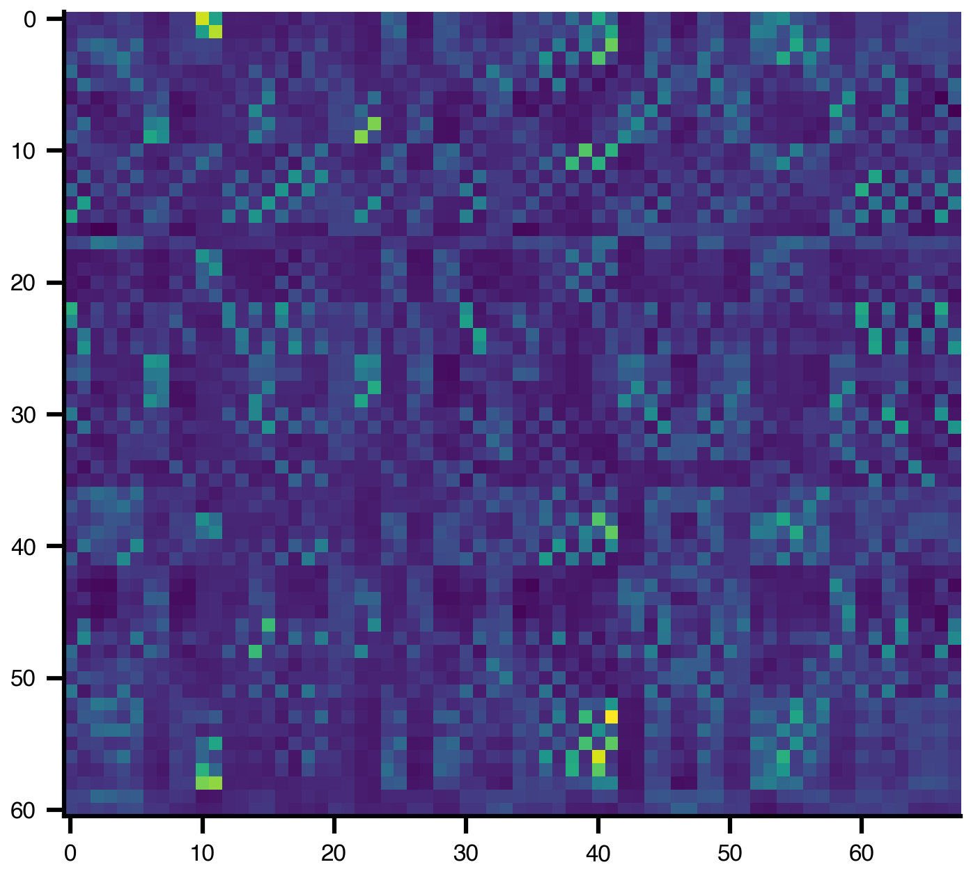

Building a projection graph

execute(format="networkx") constructs a bipartite graph connecting sensors to brain regions via thresholded gain edges. The target brain network is resolved automatically from the edge’s target_network reference — no extra argument needed:

G = sensor_net.execute(format="networkx", threshold_percentile=85)
n_s = sum(1 for _, d in G.nodes(data=True) if d["node_type"] == "sensor")
n_r = sum(1 for _, d in G.nodes(data=True) if d["node_type"] == "region")
print(f"Graph: {n_s} sensors + {n_r} regions = {G.number_of_nodes()} nodes")
print(f"Edges: {G.number_of_edges()} (gain > 85th percentile)")

Graph: 61 sensors + 68 regions = 129 nodes
Edges: 623 (gain > 85th percentile)

Every node has a pos attribute (MNI coordinates) and a color attribute (red for sensors, blue for regions), so the graph is ready for 3D rendering with bsplot:

import matplotlib.pyplot as plt
from bsplot.graph import plot_network_on_surface

fig, axes = plt.subplots(1, 2, figsize=(6, 3), layout="compressed")
for ax, view in zip(axes, ["front", "top"]):
    plot_network_on_surface(
        G,
        ax=ax,
        view=view,
        node_radius=1.5,
        node_color="auto",
        edge_radius=0.004,
        edge_color="auto",
        edge_cmap="hot",
        edge_data_key="gain",
        edge_scale={"gain": 2, "mode": "log"},
        surface_alpha=0.12,
        nodes=list(G.nodes()),
    )
    ax.set_title(view)
plt.show()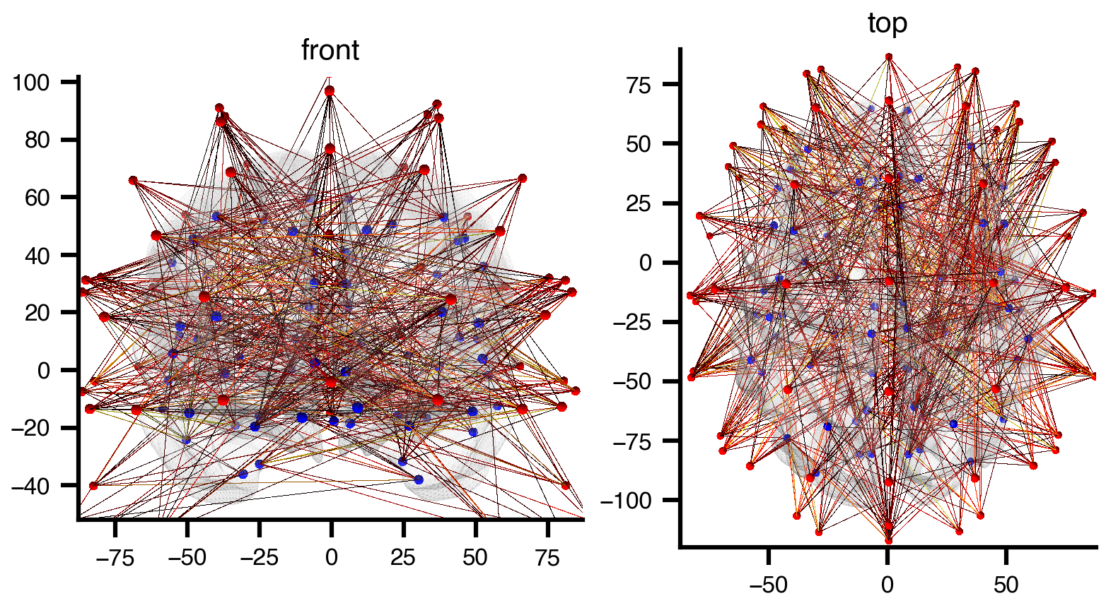

Optionally, overlay a translucent head surface from MNE’s fsaverage BEM model using extra_surfaces:

Load MNE fsaverage head surface and render with network

import mne
import nibabel as nib
from pathlib import Path

fs_dir = Path(mne.datasets.fetch_fsaverage(verbose=False))
head_surfs = mne.read_bem_surfaces(
    str(fs_dir / "bem" / "fsaverage-head.fif"), verbose=False
)
head_verts = head_surfs[0]["rr"] * 1000   # m → mm
head_tris = head_surfs[0]["tris"]

head_gifti = nib.gifti.GiftiImage()
head_gifti.add_gifti_data_array(
    nib.gifti.GiftiDataArray(
        head_verts.astype(np.float32), intent="NIFTI_INTENT_POINTSET"
    )
)
head_gifti.add_gifti_data_array(
    nib.gifti.GiftiDataArray(
        head_tris.astype(np.int32), intent="NIFTI_INTENT_TRIANGLE"
    )
)

fig, axes = plt.subplots(1, 2, figsize=(6, 3), layout="compressed")
for ax, view in zip(axes, ["front", "top"]):
    plot_network_on_surface(
        G,
        ax=ax,
        view=view,
        node_radius=1.5,
        node_color="auto",
        edge_radius=0.004,
        edge_color="auto",
        edge_cmap="hot",
        edge_data_key="gain",
        edge_scale={"gain": 12, "mode": "log"},
        surface_alpha=0.12,
        nodes=list(G.nodes()),
        extra_surfaces=[head_gifti],
        extra_colors=["wheat"],
        extra_alphas=[0.06],
    )
    ax.set_title(view)
plt.show()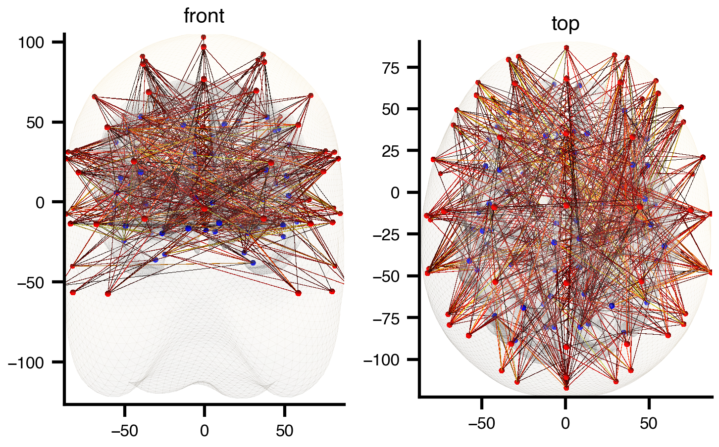

YAML structure

The sensor network YAML follows the standard Network schema with descriptor: sensors and a template edge for the gain matrix:

tvbo_class: tvbo:Network
label: EEG standard_1005 fsaverage projection
descriptor: sensors
distance_unit: mm
data_file: tpl-fsaverage_acq-EEGstandard1005_atlas-DesikanKilliany_desc-projection_sensors.h5

nodes:
  - id: 0
    label: Fp1
    position: {x: -29.44, y: 83.92, z: -6.99}
  - id: 1
    label: Fp2
    position: {x: 29.87, y: 84.90, z: -7.08}
  # ... 61 EEG channels with MNI coordinates

edges:
  - label: gain           # matrix name in HDF5
    format: dense
    directed: false
    target_network: ...DesikanKilliany_desc-SC_relmat.yaml
    dimension_labels:     # ordered column labels (68 DK cortical regions)
      - ctx-lh-bankssts
      - ctx-lh-caudalanteriorcingulate
      # ... 68 entries total

The HDF5 companion stores data and dimension scales (HDF5 §12.2) that label matrix rows and columns:

Dataset	Shape	Content
`edges/gain/data`	\((61, 68)\)	Lead-field projection matrix
`edges/gain/_dim_row_labels`	\((61,)\)	Sensor labels (dim-0 scale)
`edges/gain/_dim_col_labels`	\((68,)\)	Region labels (dim-1 scale)
`nodes/coordinates`	\((61, 3)\)	Sensor positions (MNI mm)

Reference

Constructors

Method	Use case
`Network.from_string(yaml)`	Small networks, inline YAML
`Network.from_matrix(W, L)`	Large connectomes from arrays
`Network.from_file(path)`	Load saved network (lazy arrays)
`Network.from_tvb_zip(path)`	Import TVB connectivity ZIP
`Network.from_db(name)`	Built-in normative connectome

I/O & Export

Method	Description
`net.save(path)`	Save as YAML + HDF5 (or Zarr, CSV)
`net.to_bep017(dir)`	Export to BIDS BEP017 format
`net.bids_filename`	Generate BIDS-compliant filename
`net.execute(format="tvb")`	Convert to TVB `Connectivity`
`net.execute(format="networkx", target=...)`	Build NetworkX graph (auto-resolves target for projections)

Visualization

Method	Description
`net.plot_graph()`	Force-directed graph layout
`net.plot_matrix()`	Side-by-side weight/length heatmaps
`net.plot_weights(ax)`	Weight matrix on a given axes
`net.plot_lengths(ax)`	Length matrix on a given axes
`net.plot_overview()`	Three-panel summary (graph + matrices)

Properties

Property	Returns
`net.weights_matrix`	Weight array (N × N)
`net.lengths_matrix`	Tract length array (N × N)
`net.matrix(name)`	Any named matrix (e.g. `"gain"`)
`net.number_of_nodes`	Number of regions
`net.node_labels`	List of region labels
`net.graph`	NetworkX graph (nodes have `pos` attribute)

YAML Schema

label: My Network          # Display name
descriptor: SC             # "SC" (structural) or "FC" (functional)
distance_unit: mm
time_unit: ms
data_file: my_network.h5   # HDF5 companion file

bids:                      # BIDS BEP017 entities (optional)
  bids_version: "1.10.0"
  dataset_type: derivative
  template: MNI152NLin2009cAsym
  cohort: HCPYA
  reconstruction: dTOR

nodes:
  - id: 0                  # Unique integer ID
    label: V1              # Display label
    position:              # MNI coordinates (optional)
      x: -30
      y: -80
      z: 0

edges:
  - label: weights         # Template edge (matrix name)
    format: dense           # "dense", "csr", or "coo"
    weighted: true
    valid_diagonal: false
    non_negative: true
  - label: lengths
    unit: mm
    format: dense

parcellation:              # For built-in connectomes
  atlas:
    name: DesikanKilliany
    coordinateSpace: MNI152NLin2009cAsym

tractogram:                # Source tractography dataset
  name: dTOR

normalization:             # Weight normalization equation
  rhs: "(W - W_min) / (W_max - W_min)"