PDE Simulation

TVB-O supports surface-based partial differential equations using finite element methods via scikit-fem. The PDE backend generates a self-contained implicit Euler FEM solver from a YAML experiment description, supporting triangle and tetrahedral meshes, Dirichlet boundary conditions, and constant or time-dependent source terms.

\[ \partial_t u(t,\mathbf{x}) = D\,\Delta u(t,\mathbf{x}) \quad \text{in } \Omega, \qquad u(t,\mathbf{x}) = 0 \quad \text{on } \partial\Omega \]

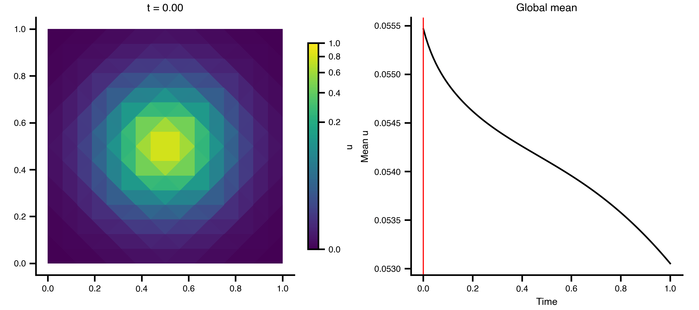
Example 1: Heat Equation on a 2D Grid

A minimal diffusion example on a unit square, using scikit-fem’s built-in mesh generators.

Step 1 — Create a triangle mesh and experiment YAML

import tempfile, os, yaml
import meshio
import numpy as np
from skfem import MeshTri
from bsplot import style
style.use("tvbo")

# Generate a symmetric unit-square triangulation
mesh = MeshTri.init_symmetric().refined(3)
tmpdir = tempfile.mkdtemp()
mesh_path = os.path.join(tmpdir, "unit_square.msh")
meshio.Mesh(points=mesh.p.T, cells=[("triangle", mesh.t.T)]).write(mesh_path)
print(f"Mesh: {mesh.p.shape[1]} vertices, {mesh.t.shape[1]} triangles")

# Write experiment YAML
exp_dict = {
    "label": "Heat equation on unit square",
    "field_dynamics": {
        "label": "Heat / diffusion equation",
        "mesh": {
            "label": "unit_square",
            "element_type": "triangle",
            "mesh_file": mesh_path,
        },
        "parameters": {"D": {"name": "D", "value": 0.01}},
        "state_variables": [
            {
                "name": "u",
                "label": "Temperature",
                "initial_value": 0.0,
                "boundary_conditions": [
                    {
                        "label": "Zero Dirichlet",
                        "bc_type": "Dirichlet",
                        "value": {"rhs": "0"},
                    }
                ],
                "equation": {"lhs": "u_t", "rhs": "D * laplacian(u)"},
            }
        ],
        "operators": [
            {"label": "Diffusion", "operator_type": "laplacian", "coefficient": "D"}
        ],
        "solver": {
            "label": "FEM implicit Euler",
            "discretization": "FEM",
            "time_integrator": "implicit Euler",
            "dt": 0.01,
        },
    },
    "integration": {"duration": 1.0},
}
yaml_path = os.path.join(tmpdir, "pde_heat_2d.yaml")
with open(yaml_path, "w") as f:
    yaml.dump(exp_dict, f)

Mesh: 145 vertices, 256 triangles

Step 2 — Run the simulation

from tvbo import SimulationExperiment

exp = SimulationExperiment.from_file(yaml_path)
ns = exp.execute("pde")
nodes = ns["meta"]["nodes"]
x, y = nodes[0], nodes[1]

# Gaussian bump initial condition centred at (0.5, 0.5)
u0 = np.exp(-((x - 0.5)**2 + (y - 0.5)**2) / 0.02)

ts = exp.run("pde", u0=u0)
print(f"TimeSeries: {ts.data.shape}  (time, state_var, nodes)")
print(f"Time: {ts.time[0]:.2f} to {ts.time[-1]:.2f}, dt={ts.time[1] - ts.time[0]:.3f}")

TimeSeries: (101, 1, 145)  (time, state_var, nodes)
Time: 0.00 to 1.00, dt=0.010

Step 3 — Animate the diffusion

import matplotlib.pyplot as plt
import matplotlib.tri as mtri
from matplotlib.colors import PowerNorm
from matplotlib.animation import PillowWriter
from IPython.display import Image

triang = mtri.Triangulation(x, y, ns["meta"]["cells"].T)
n_frames = ts.data.shape[0]
vmin, vmax = 0, float(np.max(ts.data))
norm = PowerNorm(gamma=0.3, vmin=vmin, vmax=vmax)

fig, (ax_mesh, ax_ts) = plt.subplots(1, 2, figsize=(9, 4), layout="compressed")

# Add a fixed colorbar (norm is constant across frames)
import matplotlib.cm as cm
sm = cm.ScalarMappable(norm=norm, cmap="viridis")
fig.colorbar(sm, ax=ax_mesh, label="u", shrink=0.8)

def update_2d(frame):
    ax_mesh.clear()
    ax_mesh.tripcolor(triang, np.asarray(ts.data[frame, 0, :]), norm=norm, cmap="viridis")
    ax_mesh.set_title(f"t = {ts.time[frame]:.2f}")
    ax_mesh.set_aspect("equal")

    ax_ts.clear()
    ax_ts.plot(ts.time, np.asarray(ts.data[:, 0, :]).mean(axis=1), color="black")
    ax_ts.axvline(ts.time[frame], color="red", lw=1)
    ax_ts.set_xlabel("Time")
    ax_ts.set_ylabel("Mean u")
    ax_ts.set_title("Global mean")

os.makedirs("_output", exist_ok=True)
from matplotlib.animation import FuncAnimation
anim = FuncAnimation(fig, update_2d, frames=n_frames, interval=100)
anim.save("_output/pde_heat_2d.gif", writer="pillow", fps=10)
plt.close()

Heat equation diffusion on unit square

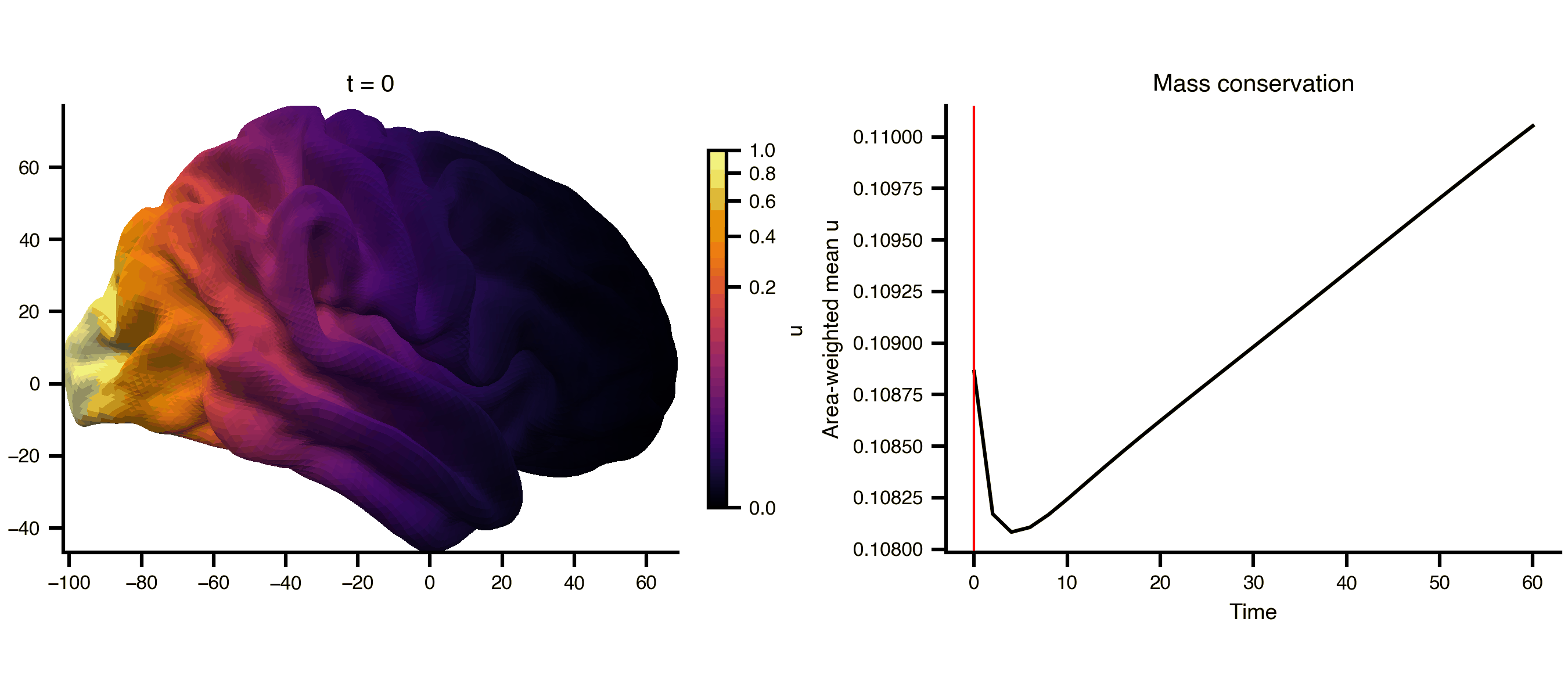
Example 2: Cortical Surface Diffusion

Diffusion on a cortical surface mesh (fsLR 32k), using the mesh_file attribute to reference an external GIFTI file directly. The cortical midthickness surface is a closed manifold (no boundary), so the Dirichlet BC has no effect and total mass is conserved — the field spreads but doesn’t decay.

Setup and run

import templateflow.api as tfa
import nibabel as nib

# Get RH midthickness surface from templateflow
mesh_gii = str(tfa.get(template="fsLR", density="32k", suffix="midthickness", hemi="R", desc=None))

# D=50 gives visible spreading on mm-scale cortical mesh (edge ≈ 1.6 mm)
exp_cortex = {
    'label': 'Cortical surface diffusion',
    'field_dynamics': {
        'label': 'Heat/diffusion equation',
        'mesh': {
            'label': 'cortex_rh',
            'element_type': 'triangle',
            'mesh_file': mesh_gii,
            'mesh_format': 'gifti',
        },
        'parameters': {'D': {'name': 'D', 'value': 50.0}},
        'state_variables': [{
            'name': 'u', 'label': 'u',
            'initial_value': 0.0,
            'boundary_conditions': [{'label': 'Zero Dirichlet', 'bc_type': 'Dirichlet', 'value': {'rhs': '0'}}],
            'equation': {'lhs': 'u_t', 'rhs': 'D * laplacian(u)'},
        }],
        'operators': [{'label': 'Diffusion', 'operator_type': 'laplacian', 'coefficient': 'D'}],
        'solver': {'label': 'FEM IE', 'discretization': 'FEM', 'time_integrator': 'implicit Euler', 'dt': 2.0},
    },
    'integration': {'duration': 60},
}

tmpdir2 = tempfile.mkdtemp()
yaml_path2 = os.path.join(tmpdir2, 'pde_cortex.yaml')
with open(yaml_path2, 'w') as f:
    yaml.dump(exp_cortex, f)

exp2 = SimulationExperiment.from_file(yaml_path2)

# Load mesh for initial condition
gi = nib.load(mesh_gii)
vertices = gi.darrays[0].data

# Gaussian centred at the most posterior vertex (occipital pole), σ ≈ 45 mm
seed_idx = np.argmin(vertices[:, 1])
seed = vertices[seed_idx]
dist_sq = np.sum((vertices - seed)**2, axis=1)
u0 = np.exp(-dist_sq / 2000)

ts2 = exp2.run("pde", u0=u0)
print(f"Cortical PDE: {ts2.data.shape}, {vertices.shape[0]} vertices")

Cortical PDE: (31, 1, 32492), 32492 vertices

Animate with bsplot

from matplotlib.colors import PowerNorm
from bsplot.surface import plot_surf
from bsplot.animate import animate_axes


n_frames = ts2.data.shape[0]
vmax2 = float(np.max(ts2.data))
norm2 = PowerNorm(gamma=0.3, vmin=0, vmax=vmax2)

fig2, (ax_surf, ax_ts) = plt.subplots(1, 2, figsize=(9, 4), layout="compressed")

# Add a fixed colorbar
import matplotlib.cm as cm
sm2 = cm.ScalarMappable(norm=norm2, cmap="inferno")
fig2.colorbar(sm2, ax=ax_surf, label="u", shrink=0.8)

# Area-weighted mean (conserved on closed surface), not arithmetic mean
faces = gi.darrays[1].data
v0, v1, v2 = vertices[faces[:, 0]], vertices[faces[:, 1]], vertices[faces[:, 2]]
tri_areas = 0.5 * np.linalg.norm(np.cross(v1 - v0, v2 - v0), axis=1)
vertex_areas = np.zeros(len(vertices))
for k in range(3):
    np.add.at(vertex_areas, faces[:, k], tri_areas / 3)
global_mean = np.array([
    (vertex_areas * np.asarray(ts2.data[t, 0, :])).sum() / vertex_areas.sum()
    for t in range(n_frames)
])

def cortex_update(frame, ax, axis_idx, context):
    ax.clear()
    if axis_idx == 0:
        overlay = np.asarray(context["ts"].data[frame, 0, :])
        plot_surf(
            context["gii"], overlay=overlay,
            hemi="rh", view="lateral", ax=ax,
            cmap="inferno", norm=context["norm"],
        )
        ax.set_title(f"t = {context['ts'].time[frame]:.0f}")
        return []
    else:
        ax.plot(context["ts"].time, context["mean"], color="black")
        ax.axvline(context["ts"].time[frame], color="red", lw=1)
        ax.set_xlabel("Time")
        ax.set_ylabel("Area-weighted mean u")
        ax.set_title("Mass conservation")
        return []

ctx = {"ts": ts2, "gii": gi, "norm": norm2, "mean": global_mean}
anim2 = animate_axes(fig2, [ax_surf, ax_ts], n_frames=n_frames,
                     update_fn=cortex_update, context=ctx, interval=200)
anim2.save("_output/pde_cortex.gif", writer="pillow", fps=6)
plt.close()

Cortical surface diffusion

Numerical details

The backward-Euler FEM update assembles mass (\(M\)) and stiffness (\(K\)) matrices over linear triangular elements and solves, at each step:

\[ (M + \Delta t \, D \, K) \, \mathbf{u}^{n+1} = M \, \mathbf{u}^{n} + \Delta t \, M \, \mathbf{f}^{n} \]

Mesh Support

The Mesh class supports two ways to reference mesh geometry:

Attribute	Description
mesh_file	Path to external mesh file (GIFTI, VTK, MSH, FreeSurfer, etc.)
mesh_format	Explicit format override (gifti, freesurfer, meshio). Auto-detected from extension if omitted
dataLocation	Legacy attribute — still works, supports prefix syntax (gifti:path/to/file.gii)

Supported mesh formats:

Format	Extensions	Loader
GIFTI	.gii, .surf.gii	nibabel
FreeSurfer	.pial, .white, .inflated	nibabel
Gmsh	.msh	meshio
VTK	.vtk, .vtu	meshio
Wavefront OBJ	.obj	meshio
PLY	.ply	meshio

Generated Code

The PDE backend generates a self-contained scikit-fem solver from the YAML specification:

code = exp.render_code("pde")
print(code[:500])

The generated module contains:

Function	Purpose
_load_mesh()	Load GIFTI, FreeSurfer, or meshio mesh formats
build()	Assemble mass and stiffness matrices, return solver closures
solve_pde()	Implicit Euler timestepping with optional source terms
visualize()	Matplotlib field plot via scikit-fem

Schema Classes

Class	Purpose
PDE	Top-level PDE problem definition
SpatialDomain	Coordinate space and geometry
Mesh	Triangle/tetrahedron element mesh with mesh_file/mesh_format
FieldStateVariable	Spatially distributed state variable
DifferentialOperator	Gradient, divergence, laplacian, curl
BoundaryCondition	Dirichlet, Neumann, Robin, Periodic
PDESolver	FEM/FDM/FVM discretization config

See Also

• Simulation Experiments — the 'pde' backend
• Code Generation & Export — render_code('pde')