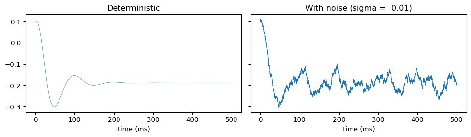
Stochastic integration uses the Heun method (stochastic Heun-Euler). Set method: heun for best accuracy with noise.
Stochastic time-varying parameter inputs
Some models drive a parameter with a random process instead of (or in addition to) Wiener noise on the state. The classical example is Jansen-Rit’s p: an external pulse density resampled at every integration step from a uniform distribution. TVBO expresses this declaratively by attaching a distribution to the parameter with axis: time.
YAML schema
parameters:p:name: pvalue:220 # constant fallback used by non-stochastic backendsunit: s^-1shape:"(n_nodes,)" # optional; (n_nodes,) ⇒ per-node trajectorydistribution:name: Uniform # Uniform | Gaussian / Normal | TruncatedNormaldomain:{lo:120,hi:320}seed:42 # optional; defaults to 42axis: time # ⇐ key: "Resample every integration timestep"
The axis: time value of SamplingAxis marks the parameter as a stochastic time-varying input (the alternative axis: space declares heterogeneous-by-node sampling, see Heterogeneous Node Dynamics).
What the tvboptim backend generates
For each axis: time parameter, the template emits:
A pre-generated trajectory of length \(\lceil t_1/\Delta t \rceil + 2\), sampled via jax.random.uniform / normal / truncated_normal and stored on state.dynamics._stoch_<name> once at the start of the run:
A per-step lookup inside dfun that reads the current sample by index:
p = params._stoch_p[jnp.int32(jnp.clip(t * inv_dt, 0, ...))]
A _freeze_step_time patch on the solver. Multi-stage methods (RK4, Heun) evaluate the dfun at sub-step times \(t,\, t + \Delta t/2,\,
t + \Delta t\). The freeze ensures all sub-evaluations within one step read the same noise sample — the input is sampled once per integration step, not interpolated across sub-stages.
Distribution names and parameterisation
name
tvboptim sampler
Mapping from domain
Uniform
jax.random.uniform
minval=lo, maxval=hi
Gaussian / Normal
jax.random.normal
mean = value, std = (hi - lo)/4
TruncatedNormal
jax.random.truncated_normal
mean = value, std = (hi - lo)/4, clipped to [lo, hi]
For Gaussian/TruncatedNormal, the fallbackvalue (used by non-stochastic backends and as the centre of the distribution) is the parameter’s value: field, not the domain midpoint.
Per-node vs scalar
The trajectory shape is determined by parameters.<name>.shape:
shape: "(n_nodes,)" ⇒ (n_steps, n_nodes) — independent draw per node per step.
otherwise ⇒ (n_steps,) — one draw per step, broadcast to all nodes.
Reproducibility
The seed lives on the distribution itself (distribution.seed). The template wires it into jax.random.key(<seed>) at run time. Two runs with the same seed produce bit-identical trajectories on the same backend; seeds do not transfer between backends (tvboptim ↔︎ jax ↔︎ tvb use different RNGs).
Comparing to deterministic backends
Only tvboptim currently honours distribution: { axis: time }. The jax and tvb codegen treats the parameter as the constant value. To run a deterministic baseline across all three backends, replace the distribution with the domain midpoint as a constant:
for p in exp.dynamics.parameters.values():if p.distribution isnotNone: dom = p.distribution.domain p.value = (float(dom.lo) +float(dom.hi)) /2.0 p.distribution =None
This pattern, plus stripping integration.noise, gives bit-comparable output across backends — see Cross-Backend Numerical Parity.