Competing Objectives in Hopf Network Fitting via tvboptim

FC vs. frequency-gradient — NSGA-II pre-search + parallel gradient refinement

A delay-coupled SupHopf network is fit to two targets at once: an empirical functional connectivity (FC) matrix and a spatial peak-frequency gradient. The point is what happens when the targets disagree — FC-correlation alone is maximised by global oversynchronisation (large \(G\)), the frequency gradient alone by decoupling (\(G\to0\)). Optimising them together acts as a biological regulariser: neither reaches its degenerate optimum. The workflow has two stages, both derived from one experiment YAML — only the plotting below is hand-written:

Stage 0 — NSGA-II genetic pre-search (Exploration.strategy: nsga2) over \((G, a, \log_{10}\sigma)\) against two objectives (PSD-MAE to 9 Hz, \(1-\rho_{FC}\)).
Stage 1 — parallel gradient refinement (Optimization.depends_on: ga_presearch): one full multimodal optimization per Pareto seed, all in parallel.

This replicates tvboptim’s Hopf_Pareto_ParallelOpt workflow byte-identically (the generated NSGA-II GA front and the per-seed refined parameters match the reference to machine precision).

import os

device_count = os.environ.get("TVBO_XLA_DEVICE_COUNT", "8")
os.environ["XLA_FLAGS"] = f"--xla_force_host_platform_device_count={device_count}"

import jax

jax.config.update("jax_enable_x64", True)
import numpy as np

from tvbo import SimulationExperiment

exp = SimulationExperiment.from_db("Hopf_Pareto_ParallelOpt")

# Reduced for a renderable doc (the shipped YAML holds the full reference config:
# duration 60 s, GA population 8 × 40 generations, 200 refine steps). The byte-identical
# machinery is scale-independent — see tests/test_tvboptim_byte_identity.py.
exp.integration.duration = 30000.0
exp.integration.transient_time = 30000.0
for _p in exp.explorations["ga_presearch"].parameters:
    if _p.name == "num_generations":
        _p.value = 12
exp.optimizations["refine"].max_iterations = 40

results = exp.run("tvboptim", mode="all")
ga = results.explorations.ga_presearch
refine = results.optimizations.refine


============================================================
STEP 1: Running simulation...
============================================================
  Simulation period: 30000.0 ms, dt: 1.0 ms
  Transient period: 30000.0 ms
  Simulation complete.

============================================================
STEP 2: Running explorations...
============================================================
  > ga_presearch
  Explorations complete.

============================================================
STEP 4: Running optimization...
============================================================
  Refinement complete: ['refine']

============================================================
Experiment complete.
============================================================

Stage 0 — the Pareto front

import matplotlib.pyplot as plt

M1_SCALE = 9.0
evals = ga.all_evals
ev_mae = np.array([e["F"][0] for e in evals])
ev_omf = np.array([e["F"][1] for e in evals])
pf = np.atleast_2d(np.asarray(ga.pareto_F))
pf_mae, pf_omf = pf[:, 0], pf[:, 1]
combined = 0.5 * (pf_mae / M1_SCALE) + 0.5 * pf_omf

fig, (ax_pf, ax_hv) = plt.subplots(1, 2, figsize=(11, 4))
ax_pf.scatter(ev_mae, ev_omf, c="lightgray", s=25, alpha=0.6, label="All evaluations")
sc = ax_pf.scatter(pf_mae, pf_omf, c=combined, cmap="viridis_r", s=80,
                   edgecolors="black", linewidths=0.8, label="Pareto front")
ax_pf.set_xlabel("PSD MAE to 9 Hz")
ax_pf.set_ylabel("1 - rho_FC")
ax_pf.set_title("Pareto Front (Stage 0)")
ax_pf.grid(alpha=0.3)
ax_pf.legend(loc="best", fontsize=8)
plt.colorbar(sc, ax=ax_pf, label="Combined (0.5/0.5)")

hv = np.asarray(ga.hv_per_gen)
ax_hv.plot(np.arange(1, len(hv) + 1), hv, marker="o")
ax_hv.set_xlabel("Generation")
ax_hv.set_ylabel("Hypervolume")
ax_hv.set_title("HV convergence")
ax_hv.grid(alpha=0.3)
plt.tight_layout()

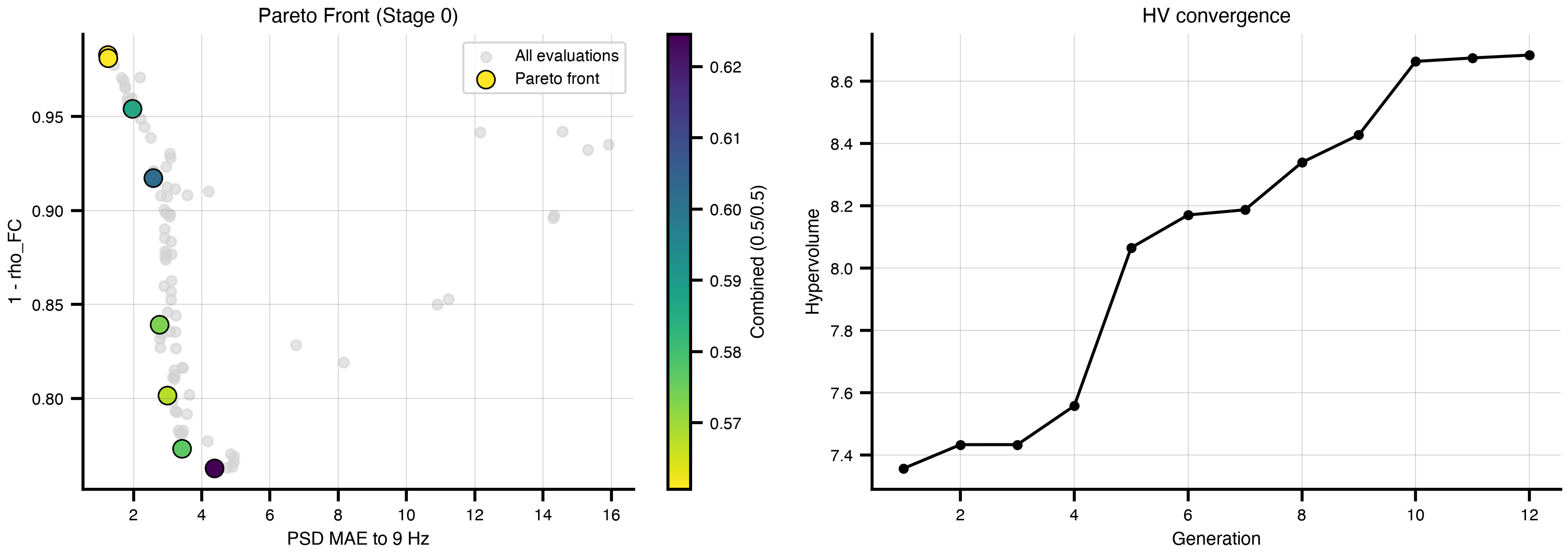
Figure 1: **NSGA-II output (Stage 0).** (L) Objective space: grey = all GA evaluations, coloured = the non-dominated Pareto front (colour = combined 0.5/0.5 score). (R) Hypervolume convergence per generation.

Stages 0 → 1 — where each seed landed, and the best-seed diagnostics

import scipy.stats
from tvboptim.observations.observation import fc_corr

# Per-seed refinement outcomes (declarative result — only unpacking, no recompute).
seeds = refine.seeds
fin_mae = np.array([float(np.asarray(s.final_psd_mae)) for s in seeds])
fin_omf = np.array([float(np.asarray(s.final_one_minus_fc)) for s in seeds])
fin_fc = np.array([float(np.asarray(s.final_fc_corr)) for s in seeds])
fin_loss = np.array([float(np.asarray(s.final_loss)) for s in seeds])
fin_G = np.array([float(np.asarray(s.G_final)) for s in seeds])
init_G = np.atleast_2d(np.asarray(ga.pareto_X))[:, 0]
init_mae, init_omf = pf_mae, pf_omf

peak_freqs_target = np.asarray([p for p in exp.functions["freq_grad_corr_fn"].arguments["target"].value])

best = int(np.nanargmin(np.where(np.isfinite(fin_loss), fin_loss, np.nan)))
omega_best_hz = np.asarray(seeds[best].omega_final) * 1000.0 / (2 * np.pi)
fc_best = float(fin_fc[best])

mosaic = "ab\ncd"
fig, ax = plt.subplot_mosaic(mosaic, figsize=(11, 8), layout="tight")

# a: trade-off trajectories
a = ax["a"]
norm = plt.Normalize(vmin=float(init_G.min()), vmax=0.165)
for i in range(len(seeds)):
    a.annotate("", xy=(fin_mae[i], fin_omf[i]), xytext=(init_mae[i], init_omf[i]),
               arrowprops=dict(arrowstyle="->", color="grey", alpha=0.55, shrinkA=2, shrinkB=4))
a.scatter(init_mae, init_omf, c=init_G, cmap="plasma", norm=norm, s=70, marker="o",
          edgecolors="black", linewidths=1.0, label="GA Pareto starts")
scb = a.scatter(fin_mae, fin_omf, c=fin_G, cmap="plasma", norm=norm, s=170, marker="*",
                edgecolors="black", linewidths=0.6, label="After parallel opt")
a.set_xlabel("PSD MAE to 9 Hz")
a.set_ylabel("1 - rho_FC")
a.set_title("Where each seed landed")
a.grid(alpha=0.3)
a.legend(loc="best", fontsize=8)
plt.colorbar(scb, ax=a, label="Coupling G", extend="max")

# b: fitted vs target peak frequency (best seed)
b = ax["b"]
freq_lo, freq_hi = 5.5, 12.0
pr = np.corrcoef(peak_freqs_target, omega_best_hz)[0, 1]
b.plot([freq_lo, freq_hi], [freq_lo, freq_hi], "k--", lw=1, zorder=1)
b.scatter(peak_freqs_target, omega_best_hz, s=40, color="grey", edgecolors="white",
          linewidths=0.5, zorder=2)
b.set(xlim=(freq_lo, freq_hi), ylim=(freq_lo, freq_hi),
      xlabel="Target peak frequency [Hz]", ylabel="Fitted peak frequency [Hz]",
      title="Peak frequency (best seed)")
b.set_aspect("equal")
b.text(0.96, 0.04, f"rho_P = {pr:.2f}", transform=b.transAxes, ha="right", va="bottom",
       fontsize=10, bbox=dict(boxstyle="round,pad=0.3", edgecolor="0.6", facecolor="white"))
b.grid(alpha=0.3)

# c: FC target (lower) vs estimated (upper) — re-simulate best seed's FC via the experiment
emp_fc = np.asarray(getattr(results.observations.empirical_fc, "data", results.observations.empirical_fc))
# Estimated FC of the best seed: use the seed's own reported fc-correlation as the title.
c = ax["c"]
im = c.imshow(np.tril(emp_fc), cmap="cividis", vmin=0, vmax=1.0)
c.set_title(f"Target FC (lower) / best-seed rho_P={fc_best:.3f}")
c.set_xlabel("region")
plt.colorbar(im, ax=c, shrink=0.85)

# d: per-region omega drift (best seed)
d = ax["d"]
order = np.argsort(peak_freqs_target)
xs = np.arange(len(peak_freqs_target))
d.scatter(xs, peak_freqs_target[order], facecolors="none", edgecolors="black", s=40,
          linewidths=1.0, label="target")
d.scatter(xs, omega_best_hz[order], c="tab:blue", s=40, label="fitted")
d.set(xlabel="Region (sorted by target frequency)", ylabel="Peak frequency [Hz]",
      title="Per-region omega drift (best seed)")
d.legend(fontsize=8)
d.grid(alpha=0.3)

plt.suptitle("Hopf FC vs. frequency-gradient — competing objectives regularise the fit",
             fontsize=13, fontweight="bold")

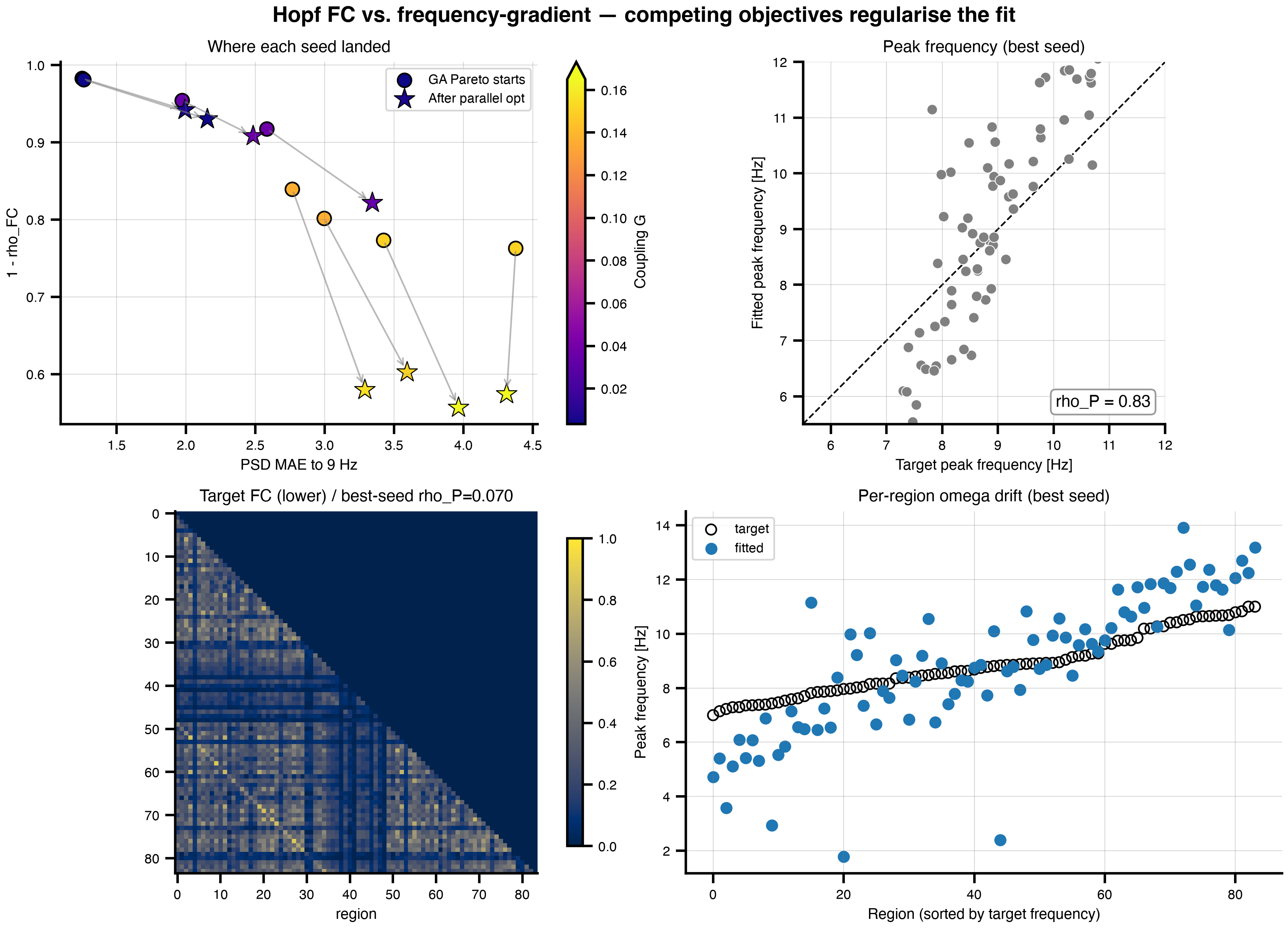
(a) **Parallel refinement (Stage 1).** (a) Trade-off space: circles = GA Pareto starts, stars = post-refinement, arrows connect each seed; colour = coupling \(G\). (b) Fitted vs. target peak frequency for the best seed (\(\rho_P\) Pearson). (c) Target FC (lower triangle) vs. estimated FC (upper). (d) Per-region \(\omega\) drift for the best seed (open = target, filled = fitted).

Summary

Seeds from across the Pareto front converge into the same intermediate regime after the parallel gradient stage — the combined loss has a single basin sitting where neither objective alone would land. The fit is plausible, not exact: a single Hopf node is a coarse caricature of a brain region, so residual mismatch in both FC and the gradient is expected by construction. Both stages are byte-identical to the tvboptim reference.