Ex18: Goldman-Hodgkin-Katz

GHK current equation for ion channel permeability with calcium dynamics

Model: GHK Current Equation

The Goldman-Hodgkin-Katz flux equation provides a more physically accurate description of ion channel current than the simple Ohmic (\(g(V-E)\)) model, accounting for ionic concentrations on both sides of the membrane:

\[I = P \cdot z^2 \cdot \frac{F^2 V}{RT} \cdot \frac{[\text{ion}]_i - [\text{ion}]_o \exp(-zFV/RT)}{1 - \exp(-zFV/RT)}\]

This example uses a Hodgkin-Huxley cell with Na, K, and Ca channels. The calcium current uses channelDensityGHK with a permeability instead of condDensity/erev, and includes an exponentially decaying calcium pool (fixedFactorConcentrationModel). The Ca gate uses q10Fixed with a hardcoded time factor.

---

1. Define HH+GHK Cell in TVBO

from tvbo import SimulationExperiment

exp = SimulationExperiment.from_string("""
label: "NeuroML Ex18: HH with GHK"
dynamics:
  name: na_k_ca
  iri: neuroml:cell
  parameters:
    diameter:           { value: 1.0 }
    length:             { value: 10.0 }
    specificCapacitance: { value: 1.0, unit: uF_per_cm2 }
    initMembPotential:  { value: -65.0, unit: mV }
    spikeThresh:        { value: 0, unit: mV }
    resistivity:        { value: 0.1, unit: kohm_cm }
    network_temperature: { value: 16.3, unit: degC }
  components:
    # ── Na channel ──
    na_chan:
      name: na_chan
      iri: neuroml:ionChannelHH
      parameters:
        conductance: { value: 10, unit: pS }
        species:     { description: na }
        condDensity: { value: 0.12, unit: S_per_cm2 }
        erev:        { value: 50.799202, unit: mV }
        ion:         { description: na }
      components:
        m:
          name: m
          iri: neuroml:gateHHrates
          parameters:
            instances: { value: 3 }
          components:
            q10Settings:
              name: q10Settings
              iri: neuroml:q10ExpTemp
              parameters:
                q10Factor:        { value: 3 }
                experimentalTemp: { value: 6.3, unit: degC }
            forwardRate:
              name: forwardRate
              iri: neuroml:HHExpLinearRate
              parameters:
                rate:     { value: 1, unit: per_ms }
                midpoint: { value: -40, unit: mV }
                scale:    { value: 10, unit: mV }
            reverseRate:
              name: reverseRate
              iri: neuroml:HHExpRate
              parameters:
                rate:     { value: 4, unit: per_ms }
                midpoint: { value: -65, unit: mV }
                scale:    { value: -18, unit: mV }
        h:
          name: h
          iri: neuroml:gateHHrates
          parameters:
            instances: { value: 1 }
          components:
            q10Settings:
              name: q10Settings
              iri: neuroml:q10ExpTemp
              parameters:
                q10Factor:        { value: 3 }
                experimentalTemp: { value: 6.3, unit: degC }
            forwardRate:
              name: forwardRate
              iri: neuroml:HHExpRate
              parameters:
                rate:     { value: 0.07, unit: per_ms }
                midpoint: { value: -65, unit: mV }
                scale:    { value: -20, unit: mV }
            reverseRate:
              name: reverseRate
              iri: neuroml:HHSigmoidRate
              parameters:
                rate:     { value: 1, unit: per_ms }
                midpoint: { value: -35, unit: mV }
                scale:    { value: 10, unit: mV }
    # ── K channel ──
    k_chan:
      name: k_chan
      iri: neuroml:ionChannelHH
      parameters:
        conductance: { value: 10, unit: pS }
        species:     { description: k }
        condDensity: { value: 0.036, unit: S_per_cm2 }
        erev:        { value: -77.0, unit: mV }
        ion:         { description: k }
      components:
        n:
          name: n
          iri: neuroml:gateHHrates
          parameters:
            instances: { value: 4 }
          components:
            q10Settings:
              name: q10Settings
              iri: neuroml:q10ExpTemp
              parameters:
                q10Factor:        { value: 3 }
                experimentalTemp: { value: 6.3, unit: degC }
            forwardRate:
              name: forwardRate
              iri: neuroml:HHExpLinearRate
              parameters:
                rate:     { value: 0.1, unit: per_ms }
                midpoint: { value: -55, unit: mV }
                scale:    { value: 10, unit: mV }
            reverseRate:
              name: reverseRate
              iri: neuroml:HHExpRate
              parameters:
                rate:     { value: 0.125, unit: per_ms }
                midpoint: { value: -65, unit: mV }
                scale:    { value: -80, unit: mV }
    # ── Ca channel (uses GHK permeability) ──
    ca_chan:
      name: ca_chan
      iri: neuroml:ionChannelHH
      parameters:
        conductance:  { value: 10, unit: pS }
        species:      { description: ca }
        permeability: { value: 2.5e-7, unit: m_per_s }
        ion:          { description: ca }
      components:
        p:
          name: p
          iri: neuroml:gateHHrates
          parameters:
            instances: { value: 2 }
          components:
            q10Settings:
              name: q10Settings
              iri: neuroml:q10Fixed
              parameters:
                fixedQ10:         { value: 0.5 }
                experimentalTemp: { value: 6.3, unit: degC }
            forwardRate:
              name: forwardRate
              iri: neuroml:HHExpLinearRate
              parameters:
                rate:     { value: 1, unit: per_ms }
                midpoint: { value: -40, unit: mV }
                scale:    { value: 10, unit: mV }
            reverseRate:
              name: reverseRate
              iri: neuroml:HHExpRate
              parameters:
                rate:     { value: 4, unit: per_ms }
                midpoint: { value: -65, unit: mV }
                scale:    { value: -18, unit: mV }
    # ── Leak channel ──
    leak:
      name: leak
      iri: neuroml:ionChannelPassive
      parameters:
        conductance: { value: 10, unit: pS }
        species:     { description: non_specific }
        condDensity: { value: 0.0003, unit: S_per_cm2 }
        erev:        { value: -53.1, unit: mV }
        ion:         { description: non_specific }
    # ── Calcium concentration model ──
    simple_decay:
      name: simple_decay
      iri: neuroml:fixedFactorConcentrationModel
      parameters:
        ion:           { description: ca }
        restingConc:   { value: 3e-6, unit: mM }
        decayConstant: { value: 1.0, unit: ms }
        rho:           { value: 3e-1, unit: mol_per_m_per_A_per_s }
        initialConcentration:    { value: 5e-6, unit: mM }
        initialExtConcentration: { value: 2, unit: mM }
    # ── Current clamp ──
    IClamp:
      name: IClamp
      iri: neuroml:pulseGenerator
      parameters:
        delay:     { value: 4, unit: ms }
        duration:  { value: 6.0, unit: ms }
        amplitude: { value: 0.005, unit: nA }
network:
  number_of_nodes: 1
integration:
  method: euler
  step_size: 0.001
  duration: 50.0
  time_scale: ms
""")
print(f"Model: {exp.dynamics.name if exp.dynamics else 'network'}")
print(f"Components: {list(exp.dynamics.modes.keys())}")

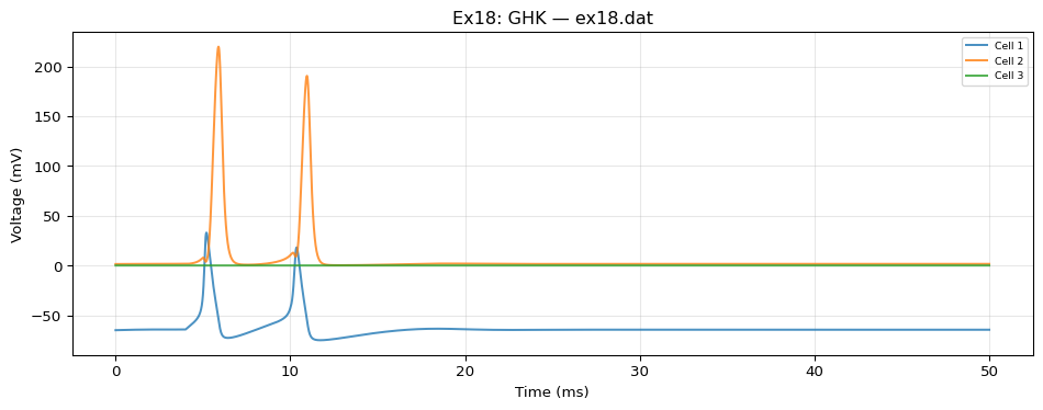
Model: na_k_ca
Components: ['IClamp', 'ca_chan', 'k_chan', 'leak', 'na_chan', 'simple_decay']

2. Render LEMS XML

xml = exp.render("lems", use_standard_types=True)
print(xml[:3000])

<Lems>
  <Target component="sim_NeuroML_Ex18__HH_with_GHK"/>

  <Include file="Cells.xml"/>
  <Include file="Networks.xml"/>
  <Include file="Inputs.xml"/>
  <Include file="Simulation.xml"/>

    <concentrationModel id="simple_decay" type="fixedFactorConcentrationModel" decayConstant="1 ms" ion="ca" restingConc="3e-06 mM" rho="0.3 mol_per_m_per_A_per_s"/>

    <ionChannelHH id="ca_chan" conductance="10 pS" species="ca">
        <gateHHrates id="p" instances="2">
            <forwardRate type="HHExpLinearRate" midpoint="-40 mV" rate="1 per_ms" scale="10 mV"/>
            <q10Settings type="q10Fixed" experimentalTemp="6.3 degC" fixedQ10="0.5"/>
            <reverseRate type="HHExpRate" midpoint="-65 mV" rate="4 per_ms" scale="-18 mV"/>
        </gateHHrates>
    </ionChannelHH>

    <ionChannelHH id="k_chan" conductance="10 pS" species="k">
        <gateHHrates id="n" instances="4">
            <forwardRate type="HHExpLinearRate" midpoint="-55 mV" rate="0.1 per_ms" scale="10 mV"/>
            <q10Settings type="q10ExpTemp" experimentalTemp="6.3 degC" q10Factor="3"/>
            <reverseRate type="HHExpRate" midpoint="-65 mV" rate="0.125 per_ms" scale="-80 mV"/>
        </gateHHrates>
    </ionChannelHH>

    <ionChannelPassive id="leak" conductance="10 pS" species="non_specific"/>

    <ionChannelHH id="na_chan" conductance="10 pS" species="na">
        <gateHHrates id="h" instances="1">
            <forwardRate type="HHExpRate" midpoint="-65 mV" rate="0.07 per_ms" scale="-20 mV"/>
            <q10Settings type="q10ExpTemp" experimentalTemp="6.3 degC" q10Factor="3"/>
            <reverseRate type="HHSigmoidRate" midpoint="-35 mV" rate="1 per_ms" scale="10 mV"/>
        </gateHHrates>
        <gateHHrates id="m" instances="3">
            <forwardRate type="HHExpLinearRate" midpoint="-40 mV" rate="1 per_ms" scale="10 mV"/>
            <q10Settings type="q10ExpTemp" experimentalTemp="6.3 degC" q10Factor="3"/>
            <reverseRate type="HHExpRate" midpoint="-65 mV" rate="4 per_ms" scale="-18 mV"/>
        </gateHHrates>
    </ionChannelHH>

    <cell id="na_k_ca">
        <morphology id="na_k_ca_morphology">
            <segment id="0" name="Soma">
                <proximal x="0.0" y="0.0" z="0.0" diameter="1.0"/>
                <distal x="0.0" y="0.0" z="10.0" diameter="1.0"/>
            </segment>
            <segmentGroup id="all">
                <member segment="0"/>
            </segmentGroup>
            <segmentGroup id="soma_group">
                <member segment="0"/>
            </segmentGroup>
        </morphology>
        <biophysicalProperties id="biophys">
            <membraneProperties>
                <channelDensityGHK permeability="2.5e-07 m_per_s" id="ca_chan_all" ionChannel="ca_chan" ion="ca"/>
                <channelDensity condDensity="0.036 S_per_cm2" id="k_chan_all" ionChannel="k_chan" erev="-77 mV" ion="k"/>
                <channelDensity condDensity="0.0003 S_per_cm2" id="leak_all" ionChannel="leak" erev="-53.1 mV

3. Run Reference

from tvbo.adapters.neuroml import run_lems_example

ref_outputs = run_lems_example("LEMS_NML2_Ex18_GHK.xml")
for name, arr in ref_outputs.items():
    print(f"  {name}: shape={arr.shape}")

  ex18.dat: shape=(50001, 4)

4. Run TVBO

result = exp.run("neuroml")
da = result.integration.data
print(f"TVBO: {da.dims}, shape={da.shape}")

TVBO: ('time', 'variable'), shape=(50001, 1)

5. Compare & Plot

from tvbo.adapters.neuroml import plot_lems_comparison
plot_lems_comparison("LEMS_NML2_Ex18_GHK.xml", ref_outputs, result.integration.data, title_prefix="Ex18")