Model: Pinsky-Rinzel CA3
The Pinsky & Rinzel (1994) two-compartment CA3 pyramidal cell model with:
Soma : Na (\(m_\infty^2 h\) ), K (\(n\) ) channels + injected currentDendrite : Ca (\(s^2\) ), K-C (\(c \cdot \chi\) ), K-AHP (\(q\) ) channelsCoupling : resistive coupling \(g_c(V_s - V_d)/(1-p)\) between compartments
10 state variables: \(V_s, V_d, Ca_d, h_s, n_s, s_d, c_d, q_d, S_i, W_i\) .
1. Define in TVBO
from tvbo import SimulationExperiment# Pinsky-Rinzel CA3 cell (pr2A variant from NeuroML Ex22) # All units: mV, ms, mS/cm², μF/cm², μA/cm² = SimulationExperiment.from_string(""" label: "NeuroML Ex22: Pinsky-Rinzel CA3" dynamics: name: PinskyRinzelCA3 parameters: iSoma: { value: 0.75 } iDend: { value: 0.0 } gLs: { value: 0.1 } gLd: { value: 0.1 } gNa: { value: 30.0 } gKdr: { value: 15.0 } gCa: { value: 10.0 } gKahp: { value: 0.8 } gKC: { value: 15.0 } gc: { value: 2.1 } eNa: { value: 60.0 } eCa: { value: 80.0 } eK: { value: -75.0 } eL: { value: -60.0 } pp: { value: 0.5 } cm: { value: 3.0 } derived_variables: alpha_ms: equation: rhs: "Piecewise((0.32/4.0, Eq(Vs, -46.9)), (0.32*(-46.9 - Vs)/(exp((-46.9 - Vs)/4.0) - 1.0), True))" beta_ms: equation: rhs: "Piecewise((0.28/5.0, Eq(Vs, -19.9)), (0.28*(Vs + 19.9)/(exp((Vs + 19.9)/5.0) - 1.0), True))" minf_s: equation: rhs: "alpha_ms / (alpha_ms + beta_ms)" alpha_hs: equation: rhs: "0.128*exp((-43.0 - Vs)/18.0)" beta_hs: equation: rhs: "4.0 / (1.0 + exp((-20.0 - Vs)/5.0))" alpha_ns: equation: rhs: "Piecewise((0.016/5.0, Eq(Vs, -24.9)), (0.016*(-24.9 - Vs)/(exp((-24.9 - Vs)/5.0) - 1.0), True))" beta_ns: equation: rhs: "0.25*exp(-1.0 - 0.025*Vs)" alpha_sd: equation: rhs: "1.6 / (1.0 + exp(-0.072*(Vd - 5.0)))" beta_sd: equation: rhs: "Piecewise((0.02/5.0, Eq(Vd, -8.9)), (0.02*(Vd + 8.9)/(exp((Vd + 8.9)/5.0) - 1.0), True))" alpha_cd: equation: rhs: "Piecewise((exp((Vd + 50.0)/11.0 - (Vd + 53.5)/27.0) / 18.975, Vd < -10.0), (2.0*exp((-53.5 - Vd)/27.0), True))" beta_cd: equation: rhs: "Piecewise((2.0*exp((-53.5 - Vd)/27.0) - alpha_cd, Vd < -10.0), (0.0, True))" alpha_qd: equation: rhs: "Min(0.00002*Cad, 0.01)" chi_d: equation: rhs: "Min(Cad/250.0, 1.0)" ICa_d: equation: rhs: "gCa*sd**2*(Vd - eCa)" state_variables: Vs: equation: rhs: "(-gLs*(Vs - eL) - gNa*minf_s**2*hs*(Vs - eNa) - gKdr*ns*(Vs - eK) + gc*(Vd - Vs)/pp + iSoma/pp) / cm" initial_value: -60.0 variable_of_interest: true Vd: equation: rhs: "(-gLd*(Vd - eL) - ICa_d - gKahp*qd*(Vd - eK) - gKC*cd*chi_d*(Vd - eK) + gc*(Vs - Vd)/(1.0 - pp) + iDend/(1.0 - pp)) / cm" initial_value: -60.0 variable_of_interest: true Cad: equation: rhs: "-0.13*ICa_d - 0.075*Cad" initial_value: 0.0 hs: equation: rhs: "alpha_hs - (alpha_hs + beta_hs)*hs" initial_value: 0.0 ns: equation: rhs: "alpha_ns - (alpha_ns + beta_ns)*ns" initial_value: 0.0 sd: equation: rhs: "alpha_sd - (alpha_sd + beta_sd)*sd" initial_value: 0.0 cd: equation: rhs: "alpha_cd - (alpha_cd + beta_cd)*cd" initial_value: 0.0 qd: equation: rhs: "alpha_qd - (alpha_qd + 0.001)*qd" initial_value: 0.0 Si: equation: rhs: "-Si/150.0" initial_value: 0.0 Wi: equation: rhs: "-Wi/2.0" initial_value: 0.0 network: number_of_nodes: 1 integration: method: euler step_size: 0.01 duration: 1500.0 time_scale: ms """ )print (f"Model: { exp. dynamics. name if exp. dynamics else 'network' } " )print (f"SVs ( { len (exp.dynamics.state_variables)} ): { list (exp.dynamics.state_variables.keys())} " )print (f"DVs ( { len (exp.dynamics.derived_variables)} ): { list (exp.dynamics.derived_variables.keys())} " )
Model: PinskyRinzelCA3
SVs (10): ['Cad', 'Si', 'Vd', 'Vs', 'Wi', 'cd', 'hs', 'ns', 'qd', 'sd']
DVs (14): ['ICa_d', 'alpha_cd', 'alpha_hs', 'alpha_ms', 'alpha_ns', 'alpha_qd', 'alpha_sd', 'beta_hs', 'beta_ms', 'beta_ns', 'beta_sd', 'chi_d', 'beta_cd', 'minf_s']
TVBO represents both compartments within a single Dynamics — somatic (\(V_s\) ) and dendritic (\(V_d\) ) are state variables coupled by \(g_c\) . This is the most complex single-cell model in the NeuroML2 examples.
2. Render LEMS XML
= exp.render("lems" )# Count lines print (f"LEMS XML: { len (xml.split(chr (10 )))} lines" )# Show TimeDerivatives for line in xml.split(' \n ' ):if 'TimeDerivative' in line:print (line.strip())
LEMS XML: 184 lines
No SEC constant is needed and TimeDerivatives use the RHS directly.
<TimeDerivative variable="Cad" value="(-0.13*ICa_d - 0.075*Cad) / SEC"/>
<TimeDerivative variable="Si" value="(-0.00666666666666667*Si) / SEC"/>
<TimeDerivative variable="Vd" value="((-ICa_d + iDend/(1.0 - pp) - gLd*(Vd - eL) + gc*(Vs - Vd)/(1.0 - pp) - gKahp*qd*(Vd - eK) - cd*chi_d*gKC*(Vd - eK))/cm) / SEC"/>
<TimeDerivative variable="Vs" value="((iSoma/pp - gLs*(Vs - eL) + gc*(Vd - Vs)/pp - gKdr*ns*(Vs - eK) - gNa*hs*minf_s^2*(Vs - eNa))/cm) / SEC"/>
<TimeDerivative variable="Wi" value="(-0.5*Wi) / SEC"/>
<TimeDerivative variable="cd" value="(alpha_cd - cd*(alpha_cd + beta_cd)) / SEC"/>
<TimeDerivative variable="hs" value="(alpha_hs - hs*(alpha_hs + beta_hs)) / SEC"/>
<TimeDerivative variable="ns" value="(alpha_ns - ns*(alpha_ns + beta_ns)) / SEC"/>
<TimeDerivative variable="qd" value="(alpha_qd - qd*(0.001 + alpha_qd)) / SEC"/>
<TimeDerivative variable="sd" value="(alpha_sd - sd*(alpha_sd + beta_sd)) / SEC"/>
3. Run Reference
from tvbo.adapters.neuroml import run_lems_example= run_lems_example("LEMS_NML2_Ex22_PinskyRinzelCA3.xml" )for name, arr in ref_outputs.items():print (f" { name} : shape= { arr. shape} " )
ex22_v.dat: shape=(150001, 3)
4. Run TVBO Version
= exp.run("neuroml" )= result.integration.dataprint (f"TVBO: { da. dims} , shape= { da. shape} " )
TVBO: ('time', 'variable'), shape=(150001, 10)
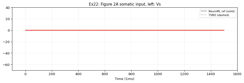
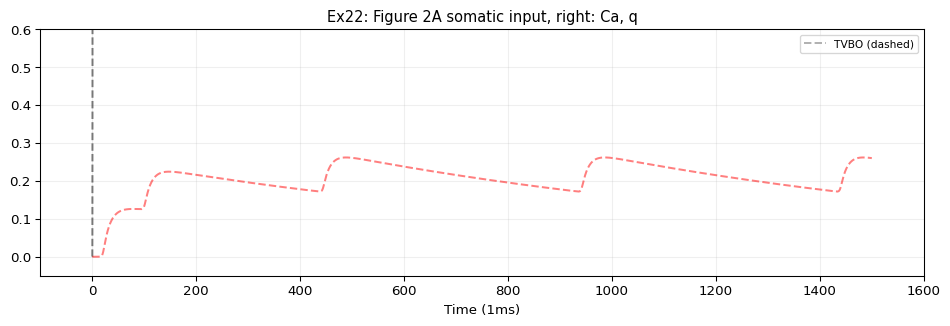
5. Compare & Plot
from tvbo.adapters.neuroml import plot_lems_comparison"LEMS_NML2_Ex22_PinskyRinzelCA3.xml" , ref_outputs, result.integration.data, title_prefix= "Ex22" )