Bayesian Inference of Stimulation & Excitability via tvboptim

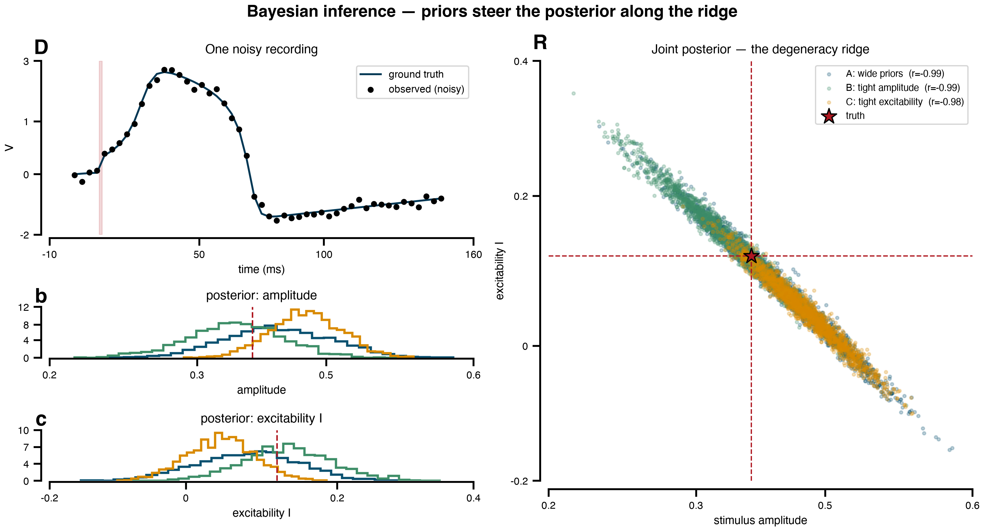
From a single noisy recording of a pulse-driven Generic2dOscillator, recover both the stimulus amplitude and the excitability I — via numpyro NUTS/MCMC. The two trade off (a degenerate ridge), so a point estimate is misleading; the posterior reports the whole ridge, and priors steer where it concentrates. Everything below is derived from one experiment YAML via exp.run(mode="inference"); only the observed-data synthesis and the plotting are hand-written.

import os

device_count = os.environ.get("TVBO_XLA_DEVICE_COUNT", "4")
os.environ["XLA_FLAGS"] = f"--xla_force_host_platform_device_count={device_count}"

import jax

jax.config.update("jax_enable_x64", True)
import numpy as np

from tvbo import SimulationExperiment

exp = SimulationExperiment.from_db("Stimulation_Bayesian_Inference")

# Synthetic ground truth (a testing concern, not the schema's): the recording is the
# forward at the declared true params (amplitude=0.4, I=0.1) plus observation noise.
rec = np.asarray(exp.run("tvboptim", mode="simulation").observations.recorded_ts.data).ravel()
observed = rec + 0.1 * np.asarray(jax.random.normal(jax.random.key(42), (rec.shape[0],)))

# Three posteriors on the SAME observation, differing only in prior widths (A/B/C).
results = exp.run("tvboptim", mode="inference", recorded_ts=observed)


============================================================
STEP 1: Running simulation...
============================================================
  Simulation period: 150.0 ms, dt: 0.2 ms
  Transient period: 0.0 ms
  Simulation complete.

============================================================
Experiment complete.
============================================================

============================================================
STEP 1: Running simulation...
============================================================
  Simulation period: 150.0 ms, dt: 0.2 ms
  Transient period: 0.0 ms
  Simulation complete.

============================================================
STEP 5: Running Bayesian inference (MCMC)...
============================================================
  Inference complete. Posteriors: ['scenario_A', 'scenario_B', 'scenario_C']

============================================================
Experiment complete.
============================================================

Results

import numpy as np
import matplotlib.pyplot as plt
import bsplot

INK, TRUE, WARN = "#003754", "#AF1821", "#AF1821"
COL = {"scenario_A": "#0a5170", "scenario_B": "#3E8E68", "scenario_C": "#d98a00"}
LAB = {"scenario_A": "A: wide priors", "scenario_B": "B: tight amplitude", "scenario_C": "C: tight excitability"}
TRUE_AMP, TRUE_I = 0.4, 0.1

post = {k: (np.asarray(v.posterior["stimulus.amplitude"]), np.asarray(v.posterior["Generic2dOscillator.I"]))
        for k, v in results.inferences.items()}

mosaic = """
DDRR
DDRR
bbRR
ccRR
"""
fig, ax = plt.subplot_mosaic(mosaic, layout="tight", figsize=(11, 6))

# D: the observed recording + ground truth
a = ax["D"]
t = np.arange(rec.shape[0]) * 0.2 * 15  # ms (subsampled every 15 at dt=0.2)
a.plot(t, rec, color=INK, lw=1.5, label="ground truth")
a.scatter(t, observed, s=14, color="k", zorder=3, label="observed (noisy)")
a.axvspan(10.0, 11.0, color=WARN, alpha=0.15)
a.set(xlabel="time (ms)", ylabel="V", title="One noisy recording")
a.legend(fontsize=8, loc="best")

# R: joint posteriors — the degeneracy ridge + prior steering
a = ax["R"]
for k, (amp, I) in post.items():
    a.scatter(amp, I, s=6, alpha=0.25, color=COL[k], label=f"{LAB[k]}  (r={np.corrcoef(amp, I)[0,1]:.2f})")
a.axvline(TRUE_AMP, color=TRUE, ls="--", lw=1)
a.axhline(TRUE_I, color=TRUE, ls="--", lw=1)
a.scatter([TRUE_AMP], [TRUE_I], color=TRUE, marker="*", s=160, edgecolors="k", zorder=5, label="truth")
a.set(xlabel="stimulus amplitude", ylabel="excitability I", title="Joint posterior — the degeneracy ridge")
a.legend(fontsize=7.5, loc="upper right")

# b, c: marginals
for key, idx, tv, lab in [("b", 0, TRUE_AMP, "amplitude"), ("c", 1, TRUE_I, "excitability I")]:
    a = ax[key]
    for k in post:
        a.hist(post[k][idx], bins=30, density=True, histtype="step", lw=1.8, color=COL[k])
    a.axvline(tv, color=TRUE, ls="--", lw=1.2)
    a.set(xlabel=lab, yticks=[], title=f"posterior: {lab}")

plt.suptitle("Bayesian inference — priors steer the posterior along the ridge", fontsize=13, fontweight="bold")
bsplot.style.format_fig(fig)

Figure 1: **Bayesian recovery of stimulus amplitude and excitability.** (L) The observed recording (points) and the noiseless ground truth (line); the red band is the pulse window. (R) Joint posteriors over amplitude and I for three prior scenarios — the strong negative correlation is the degeneracy ridge; tightening one prior slides the posterior along it (B pins amplitude → I explains; C pins I → amplitude explains). (b, c) Marginal posteriors; dashed lines mark the true values.