Ex1: Hodgkin-Huxley

Classic Hodgkin-Huxley conductance-based cell with Na, K, and leak channels

Model: Hodgkin-Huxley Point Cell

The classic 4-variable conductance-based model:

\[C\frac{dv}{dt} = -g_{Na}\,m^3\,h\,(v - E_{Na}) - g_K\,n^4\,(v - E_K) - g_L\,(v - E_L) + I_{\text{ext}}(t)\]

With gating variable kinetics: \[\frac{dx}{dt} = \alpha_x(v)(1-x) - \beta_x(v)\,x \quad \text{for } x \in \{m, h, n\}\]

The NeuroML2 example uses a pointCellCondBased with separate ion channel populations. By annotating the TVBO dynamics with iri: neuroml:pointCellCondBased and structuring the ion channels as components, TVBO emits standard NeuroML2 types that preserve the jLEMS child-before-parent RK4 evaluation order — giving exact numerical identity with the reference simulation.

---

1. Define in TVBO

from tvbo import SimulationExperiment

# HH parameters matching NeuroML2 Ex1 (hhpointcell)
# Uses `iri: neuroml:*` annotations to emit standard NeuroML types.

exp = SimulationExperiment.from_string("""
label: "NeuroML Ex1: Hodgkin-Huxley"
dynamics:
  name: HodgkinHuxley
  iri: neuroml:pointCellCondBased
  description: >
    Hodgkin-Huxley model matching NeuroML2 Ex1.
    Uses standard NeuroML types via hierarchical components.
  parameters:
    C:              { value: 10, unit: pF }
    v0:             { value: -65, unit: mV }
    thresh:         { value: 20, unit: mV }
    pulse_delay:    { value: 50, unit: ms }
    pulse_duration: { value: 50, unit: ms }
    I_amp:          { value: 0.08, unit: nA }
  components:
    passive:
      name: passive
      iri: neuroml:ionChannelPassive
      parameters:
        conductance: { value: 10, unit: pS }
        number:      { value: 300 }
        erev:        { value: -54.3, unit: mV }
    na:
      name: na
      iri: neuroml:ionChannelHH
      parameters:
        conductance: { value: 10, unit: pS }
        number:      { value: 120000 }
        erev:        { value: 50, unit: mV }
      components:
        m:
          name: m
          iri: neuroml:gateHHrates
          parameters:
            instances: { value: 3 }
          components:
            forwardRate:
              name: forwardRate
              iri: neuroml:HHExpLinearRate
              parameters:
                rate:     { value: 1, unit: per_ms }
                midpoint: { value: -40, unit: mV }
                scale:    { value: 10, unit: mV }
            reverseRate:
              name: reverseRate
              iri: neuroml:HHExpRate
              parameters:
                rate:     { value: 4, unit: per_ms }
                midpoint: { value: -65, unit: mV }
                scale:    { value: -18, unit: mV }
        h:
          name: h
          iri: neuroml:gateHHrates
          parameters:
            instances: { value: 1 }
          components:
            forwardRate:
              name: forwardRate
              iri: neuroml:HHExpRate
              parameters:
                rate:     { value: 0.07, unit: per_ms }
                midpoint: { value: -65, unit: mV }
                scale:    { value: -20, unit: mV }
            reverseRate:
              name: reverseRate
              iri: neuroml:HHSigmoidRate
              parameters:
                rate:     { value: 1, unit: per_ms }
                midpoint: { value: -35, unit: mV }
                scale:    { value: 10, unit: mV }
    k:
      name: k
      iri: neuroml:ionChannelHH
      parameters:
        conductance: { value: 10, unit: pS }
        number:      { value: 36000 }
        erev:        { value: -77, unit: mV }
      components:
        n:
          name: n
          iri: neuroml:gateHHrates
          parameters:
            instances: { value: 4 }
          components:
            forwardRate:
              name: forwardRate
              iri: neuroml:HHExpLinearRate
              parameters:
                rate:     { value: 0.1, unit: per_ms }
                midpoint: { value: -55, unit: mV }
                scale:    { value: 10, unit: mV }
            reverseRate:
              name: reverseRate
              iri: neuroml:HHExpRate
              parameters:
                rate:     { value: 0.125, unit: per_ms }
                midpoint: { value: -65, unit: mV }
                scale:    { value: -80, unit: mV }
integration:
  step_size: 0.01
  duration: 150.0
  time_scale: ms
""")
print(f"Model: {exp.dynamics.name if exp.dynamics else 'network'}")
print(f"IRI: {exp.dynamics.iri}")
print(f"Components: {list(exp.dynamics.components.keys())}")

Model: HodgkinHuxley
IRI: neuroml:pointCellCondBased
Components: ['k', 'na', 'passive']

Standard NeuroML Types

This example uses iri: neuroml:pointCellCondBased with nested components for ion channels (ionChannelHH, ionChannelPassive) and gates (gateHHrates). TVBO’s adapter detects these annotations and emits standard NeuroML2 XML elements rather than custom ComponentType definitions. This preserves the hierarchical RK4 evaluation order in jLEMS, giving exact numerical identity with the reference simulation at the original step size (0.01 ms) — no gate_rate_scale hack needed.

2. Render LEMS XML

xml = exp.render("lems")
# Show key elements of the generated XML
for line in xml.split('\n'):
    line_stripped = line.strip()
    if any(tag in line_stripped for tag in ['<ionChannel', '<gateHH', '<pointCell',
            '<channelPopulation', '<pulseGenerator', 'Rate type=', '<Include']):
        print(line_stripped)

<Include file="Cells.xml"/>
<Include file="Networks.xml"/>
<Include file="Inputs.xml"/>
<Include file="Simulation.xml"/>
<ionChannelHH id="k" conductance="10 pS">
<gateHHrates id="n" instances="4">
<forwardRate type="HHExpLinearRate" midpoint="-55 mV" rate="0.1 per_ms" scale="10 mV"/>
<reverseRate type="HHExpRate" midpoint="-65 mV" rate="0.125 per_ms" scale="-80 mV"/>
<ionChannelHH id="na" conductance="10 pS">
<gateHHrates id="h" instances="1">
<forwardRate type="HHExpRate" midpoint="-65 mV" rate="0.07 per_ms" scale="-20 mV"/>
<reverseRate type="HHSigmoidRate" midpoint="-35 mV" rate="1 per_ms" scale="10 mV"/>
<gateHHrates id="m" instances="3">
<forwardRate type="HHExpLinearRate" midpoint="-40 mV" rate="1 per_ms" scale="10 mV"/>
<reverseRate type="HHExpRate" midpoint="-65 mV" rate="4 per_ms" scale="-18 mV"/>
<ionChannelPassive id="passive" conductance="10 pS"/>
<pointCellCondBased id="HodgkinHuxley" C="10 pF" v0="-65 mV" thresh="20 mV">
<channelPopulation id="k_pop" ionChannel="k" number="36000" erev="-77 mV"/>
<channelPopulation id="na_pop" ionChannel="na" number="120000" erev="50 mV"/>
<channelPopulation id="passive_pop" ionChannel="passive" number="300" erev="-54.3 mV"/>
<pulseGenerator id="pulseGen1" delay="50 ms" duration="50 ms" amplitude="0.08 nA"/>

3. Run Reference

from tvbo.adapters.neuroml import run_lems_example

ref_outputs = run_lems_example("LEMS_NML2_Ex1_HH.xml")
for name, arr in ref_outputs.items():
    print(f"  {name}: shape={arr.shape}, t=[{arr[0,0]:.4f}, {arr[-1,0]:.4f}]")

  hh_v.dat: shape=(15001, 2), t=[0.0000, 0.1500]

4. Run TVBO Version

result = exp.run("neuroml")
da = result.integration.data
print(f"TVBO: {da.dims}, shape={da.shape}")

TVBO: ('time', 'variable'), shape=(15001, 1)

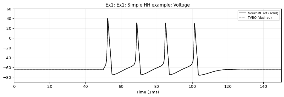
5. Compare & Plot

from tvbo.adapters.neuroml import plot_lems_comparison
plot_lems_comparison("LEMS_NML2_Ex1_HH.xml", ref_outputs, result.integration.data, title_prefix="Ex1")

---

Native Custom YAML (No IRI Dependencies)

The same Hodgkin-Huxley model, defined with full equations — no reference to standard NeuroML component types. Uses iri: extends:base* to declare LEMS base type compatibility while providing all dynamics explicitly. This makes the YAML interoperable with any backend, not just NeuroML.

6. Define Custom Version

exp_custom = SimulationExperiment.from_string("""
label: "Ex1 HH Custom"
dynamics:
  name: HodgkinHuxleyCustom
  label: customPointCellCondBased
  iri: "extends:baseCellMembPot"
  description: >
    Hodgkin-Huxley with fully explicit equations.
    All component types defined from scratch — no standard NeuroML types used.
  parameters:
    C:              { value: 10, unit: pF }
    v0:             { value: -65, unit: mV }
    thresh:         { value: 20, unit: mV }
    pulse_delay:    { value: 50, unit: ms }
    pulse_duration: { value: 50, unit: ms }
    I_amp:          { value: 0.08, unit: nA }
  state_variables:
    v:
      equation: { rhs: "(iChannels + iSyn) / C" }
      initial_value: -65.0
      unit: mV
      variable_of_interest: true
  derived_variables:
    iChannels:
      equation: { rhs: "0" }
      label: "select:populations[*]/i reduce:add"
      unit: nA
    iSyn:
      equation: { rhs: "0" }
      label: "select:synapses[*]/i reduce:add required:false"
      unit: nA
  events:
    spike:
      condition: { rhs: "v > thresh" }
  components:
    passive:
      name: passive
      label: customIonChannelHH
      iri: "extends:baseIonChannel"
      parameters:
        conductance: { value: 10, unit: pS }
        number:      { value: 300 }
        erev:        { value: -54.3, unit: mV }
      derived_variables:
        fopen:
          equation: { rhs: "1" }
        g:
          equation: { rhs: "conductance * fopen" }
          unit: nS
    na:
      name: na
      label: customIonChannelHH
      iri: "extends:baseIonChannel"
      parameters:
        conductance: { value: 10, unit: pS }
        number:      { value: 120000 }
        erev:        { value: 50, unit: mV }
      derived_variables:
        fopen:
          equation: { rhs: "1" }
          label: "select:gates[*]/fcond reduce:multiply"
        g:
          equation: { rhs: "conductance * fopen" }
          unit: nS
      components:
        m:
          name: m
          label: customGateHHrates
          iri: "extends:baseGate"
          parameters:
            instances: { value: 3 }
          state_variables:
            q:
              equation: { rhs: "(inf - q) / tau" }
              initial_value: 0.05
          derived_variables:
            alpha:
              equation: { rhs: "0" }
              label: "select:forwardRate/r"
              unit: per_ms
            beta:
              equation: { rhs: "0" }
              label: "select:reverseRate/r"
              unit: per_ms
            inf:
              equation: { rhs: "alpha / (alpha + beta)" }
            tau:
              equation: { rhs: "1 / (alpha + beta)" }
              unit: ms
            fcond:
              equation: { rhs: "q ** instances" }
          components:
            forwardRate:
              name: forwardRate
              label: customHHExpLinearRate
              iri: "extends:baseVoltageDepRate"
              parameters:
                rate:     { value: 1, unit: per_ms }
                midpoint: { value: -40, unit: mV }
                scale:    { value: 10, unit: mV }
              derived_variables:
                x:
                  equation: { rhs: "(v - midpoint) / scale" }
                r:
                  conditional: true
                  cases:
                    - condition: "x != 0"
                      equation: { rhs: "rate * x / (1 - exp(-x))" }
                    - condition: "True"
                      equation: { rhs: "rate" }
            reverseRate:
              name: reverseRate
              label: customHHExpRate
              iri: "extends:baseVoltageDepRate"
              parameters:
                rate:     { value: 4, unit: per_ms }
                midpoint: { value: -65, unit: mV }
                scale:    { value: -18, unit: mV }
              derived_variables:
                r:
                  equation: { rhs: "rate * exp((v - midpoint) / scale)" }
                  unit: per_ms
        h:
          name: h
          label: customGateHHrates
          iri: "extends:baseGate"
          parameters:
            instances: { value: 1 }
          state_variables:
            q:
              equation: { rhs: "(inf - q) / tau" }
              initial_value: 0.60
          derived_variables:
            alpha:
              equation: { rhs: "0" }
              label: "select:forwardRate/r"
              unit: per_ms
            beta:
              equation: { rhs: "0" }
              label: "select:reverseRate/r"
              unit: per_ms
            inf:
              equation: { rhs: "alpha / (alpha + beta)" }
            tau:
              equation: { rhs: "1 / (alpha + beta)" }
              unit: ms
            fcond:
              equation: { rhs: "q ** instances" }
          components:
            forwardRate:
              name: forwardRate
              label: customHHExpRate
              iri: "extends:baseVoltageDepRate"
              parameters:
                rate:     { value: 0.07, unit: per_ms }
                midpoint: { value: -65, unit: mV }
                scale:    { value: -20, unit: mV }
              derived_variables:
                r:
                  equation: { rhs: "rate * exp((v - midpoint) / scale)" }
                  unit: per_ms
            reverseRate:
              name: reverseRate
              label: customHHSigmoidRate
              iri: "extends:baseVoltageDepRate"
              parameters:
                rate:     { value: 1, unit: per_ms }
                midpoint: { value: -35, unit: mV }
                scale:    { value: 10, unit: mV }
              derived_variables:
                r:
                  equation: { rhs: "rate / (1 + exp(-(v - midpoint) / scale))" }
                  unit: per_ms
    k:
      name: k
      label: customIonChannelHH
      iri: "extends:baseIonChannel"
      parameters:
        conductance: { value: 10, unit: pS }
        number:      { value: 36000 }
        erev:        { value: -77, unit: mV }
      derived_variables:
        fopen:
          equation: { rhs: "1" }
          label: "select:gates[*]/fcond reduce:multiply"
        g:
          equation: { rhs: "conductance * fopen" }
          unit: nS
      components:
        n:
          name: n
          label: customGateHHrates
          iri: "extends:baseGate"
          parameters:
            instances: { value: 4 }
          state_variables:
            q:
              equation: { rhs: "(inf - q) / tau" }
              initial_value: 0.32
          derived_variables:
            alpha:
              equation: { rhs: "0" }
              label: "select:forwardRate/r"
              unit: per_ms
            beta:
              equation: { rhs: "0" }
              label: "select:reverseRate/r"
              unit: per_ms
            inf:
              equation: { rhs: "alpha / (alpha + beta)" }
            tau:
              equation: { rhs: "1 / (alpha + beta)" }
              unit: ms
            fcond:
              equation: { rhs: "q ** instances" }
          components:
            forwardRate:
              name: forwardRate
              label: customHHExpLinearRate
              iri: "extends:baseVoltageDepRate"
              parameters:
                rate:     { value: 0.1, unit: per_ms }
                midpoint: { value: -55, unit: mV }
                scale:    { value: 10, unit: mV }
              derived_variables:
                x:
                  equation: { rhs: "(v - midpoint) / scale" }
                r:
                  conditional: true
                  cases:
                    - condition: "x != 0"
                      equation: { rhs: "rate * x / (1 - exp(-x))" }
                    - condition: "True"
                      equation: { rhs: "rate" }
            reverseRate:
              name: reverseRate
              label: customHHExpRate
              iri: "extends:baseVoltageDepRate"
              parameters:
                rate:     { value: 0.125, unit: per_ms }
                midpoint: { value: -65, unit: mV }
                scale:    { value: -80, unit: mV }
              derived_variables:
                r:
                  equation: { rhs: "rate * exp((v - midpoint) / scale)" }
                  unit: per_ms
integration:
  step_size: 0.01
  duration: 150.0
  time_scale: ms
""")
print(f"Model: {exp_custom.dynamics.name}")
print(f"IRI: {exp_custom.dynamics.iri}")
print(f"Components: {list(exp_custom.dynamics.components.keys())}")

Model: HodgkinHuxleyCustom
IRI: extends:baseCellMembPot
Components: ['k', 'na', 'passive']

Full Custom — No NeuroML Dependencies

This version uses iri: extends:baseCellMembPot instead of iri: neuroml:pointCellCondBased. Every equation — rate functions, gating kinetics, channel conductance — is defined explicitly in the YAML. The adapter generates custom LEMS ComponentType definitions that extend base infrastructure types, achieving exact numerical identity with the standard version.

7. Run Custom Version

result_custom = exp_custom.run("neuroml")
da_custom = result_custom.integration.data
print(f"Custom: {da_custom.dims}, shape={da_custom.shape}")

Custom: ('time', 'variable'), shape=(15001, 1)

8. Compare Custom vs Reference

plot_lems_comparison(“LEMS_NML2_Ex1_HH.xml”, ref_outputs, result_custom.integration.data, title_prefix=“Ex1 Custom”)