The Virtual Brain Ontology

Welcome to tvbo!

tvbo is a Python library for defining, simulating, and analyzing dynamical systems in computational neuroscience. It combines ontology-driven knowledge representation with flexible simulation capabilities.

Core Features:

• Load: Access curated models and studies from the knowledge database
• Specify: Define dynamical systems and network models with simple specification language
• Build: Configure brain network models
• Generate: Produce optimized simulation code (Python, JAX, Julia)
• Share: Export reproducible models with standardized metadata

TVB-O GUI

Open the hosted web app to explore TVB‑O models, datasets, and simulations.

Model Browser

Browse models, parameters, and equations. Inspect relationships and components interactively.

Metadata Schema

Explore the TVB‑O metadata schema: classes, fields, and constraints used across resources.

---

Quickstart

Python Installation

pip install tvbo

For more installation options, see the Installation Guide.

Model Specification

name: LorenzAttractor
parameters:
    sigma:
        value: 10
        label: Prandtl number
    rho:
        label: Rayleigh number
        value: 28
    beta:
        value: 2.6666666666666665
state_variables:
    X:
        equation:
        lhs: \dot{X}
        rhs: sigma * (Y - X)
    Y:
        equation:
        lhs: \dot{Y}
        rhs: X * (rho - Z) - Y
    Z:
        equation:
        lhs: \dot{Z}
        rhs: X * Y - beta * Z

Generate Code

from tvbo import Dynamics, SimulationExperiment
from IPython.display import Markdown
lorenz = Dynamics(
    parameters={
        "sigma": {"value": 10.0},
        "rho": {"value": 28.0},
        "beta": {"value": 8 / 3},
    },
    state_variables={
        "X": {"equation": {"rhs": "sigma * (Y - X)"}},
        "Y": {"equation": {"rhs": "X * (rho - Z) - Y"}},
        "Z": {"equation": {"rhs": "X * Y - beta * Z"}},
    },
)

code = SimulationExperiment(dynamics=lorenz).render_code('jax')

output:

Markdown("```python" + code + "```")

import jax
from tvbo.data.types import TimeSeries
from tvbo.utils import Bunch
import jax.numpy as jnp



def cfun(weights, history, current_state, p, delay_indices, t):
    return jnp.zeros_like(current_state[0])





import jax.numpy as jnp
import jax.scipy as jsp



def dfun(current_state, t, cX, _p):
    # Parameters
    sigma = _p.sigma
    rho = _p.rho
    beta = _p.beta



    # State variables
    X = current_state[0]
    Y = current_state[1]
    Z = current_state[2]


    # Derivatives
    dX_dt = sigma*(Y - X)
    dY_dt = -Y + X*(rho - Z)
    dZ_dt = X*Y - Z*beta

    derivatives = jnp.array([dX_dt, dY_dt, dZ_dt])

    return derivatives







def integrate(state, weights, dt, params_integrate, delay_indices, external_input):
    """
    Heun Integration
    ================
    """
    t, _ = external_input
    noise = 0


    params_dfun, params_cfun, params_stimulus = params_integrate

    history, current_state = state
    stimulus = 0


    cX = jax.vmap(cfun, in_axes=(None, -1, -1, None, None, None), out_axes=-1)(weights, history, current_state, params_cfun, delay_indices, t)

    dX0 = dfun(current_state, t, cX, params_dfun)

    X = current_state



    # Calculate intermediate step X1
    X1 = X + dX0 * dt + noise + stimulus * dt

    # Calculate derivative X1
    dX1 = dfun(X1, t, cX, params_dfun)
    # Calculate the state change dX
    dX = (dX0 + dX1) * (dt / 2)
    next_state = current_state + (dX)


    return (history, next_state), next_state



import jax
import jax.numpy as jnp

def g(dt, nt, n_svar, n_nodes, n_modes, seed=0, sigma_vec=None, sigma=0.0, state=None):
    """Standard Gaussian white noise using xi ~ N(0,1).

    Returns (nt, n_svar, n_nodes, n_modes): sqrt(dt) * sigma * xi.

    - sigma_vec: optional per-state sigma (length n_svar).
    - sigma: scalar fallback when sigma_vec is None.
    - state: optional current state placeholder for future correlative noise.
    """
    key = jax.random.PRNGKey(int(seed))
    xi = jax.random.normal(key, (nt, n_svar, n_nodes, n_modes))

    if sigma_vec is not None:
        sigma_b = jnp.asarray(sigma_vec)[None, ..., None, None]
    else:
        sigma_b = jnp.asarray(sigma)

    noise = jnp.sqrt(dt) * sigma_b * xi
    return noise






def monitor_raw(time_steps, trace, params, t_offset = 0):
    dt = 0.01220703125
    return TimeSeries(time=(time_steps + t_offset) * dt, data=trace, title = "Raw")


def transform_parameters(_p):
    sigma, rho, beta = _p.sigma, _p.rho, _p.beta
    
    return _p

c_vars = jnp.array([]).astype(jnp.int32)

def kernel(state):
    # problem dimensions
    n_nodes = 1
    n_svar = 3
    n_cvar = 3
    n_modes = 1
    nh = 1

    current_state, history = (state.initial_conditions.data[-1], None) ## history = current_state

    ics = (history, current_state)
    weights = state.network.weights_matrix

    dn = jnp.arange(int(n_nodes)) * jnp.ones((int(n_nodes), int(n_nodes))).astype(jnp.int32)
    idelays = jnp.round(state.network.lengths_matrix / state.network.conduction_speed.value / state.dt).astype(jnp.int32) if state.network.conduction_speed.value > 0 else jnp.zeros((int(n_nodes), int(n_nodes)), dtype=jnp.int32)
    di = -1 * idelays - 1
    delay_indices = (di, dn)

    dt = state.dt
    nt = state.nt
    time_steps = jnp.arange(0, nt)

    # Generate batch noise using xi with per-state sigma_vec.
    # Prefer state-provided sigma_vec (supports vmapped sweeps); fallback to experiment-level constants.
    seed = getattr(state.noise, 'seed', 0) if hasattr(state.noise, 'seed') else 0
    try:
        sigma_vec_runtime = getattr(state.noise, 'sigma_vec', None)
    except Exception:
        sigma_vec_runtime = None
    sigma_vec = sigma_vec_runtime if sigma_vec_runtime is not None else jnp.array([0.,0.,0.])
    noise = g(dt, nt, n_svar, n_nodes, n_modes, seed=seed, sigma_vec=sigma_vec)


    p = transform_parameters(state.parameters.dynamics)
    params_integrate = (p, Bunch(), state.stimulus)

    op = lambda ics, external_input: integrate(ics, weights, dt, params_integrate, delay_indices, external_input)
    latest_carry, res = jax.lax.scan(op, ics, (time_steps, noise))

    trace = res


    



    trace = jnp.hstack((
        trace[:, [0], :],
        trace[:, [1], :],
        trace[:, [2], :],
        ))

    t_offset = 0
    time_steps = time_steps + 1

    
    labels_dimensions = {
        "Time": None,
        "State Variable": ['X', 'Y', 'Z'],
        "Space": ['0'],
        "Mode": ['m0'],
    }
    return TimeSeries(time=(time_steps + t_offset) * dt, data=trace, title = "Raw", sample_period=dt, labels_dimensions=labels_dimensions)

Run Dynamics

from tvbo import Dynamics, SimulationExperiment

lorenz = Dynamics(
    parameters={
        "sigma": {"value": 10.0},
        "rho": {"value": 28.0},
        "beta": {"value": 8 / 3},
    },
    state_variables={
        "X": {"equation": {"rhs": "sigma * (Y - X)"}},
        "Y": {"equation": {"rhs": "X * (rho - Z) - Y"}},
        "Z": {"equation": {"rhs": "X * Y - beta * Z"}},
    },
)

SimulationExperiment(dynamics=lorenz).run(duration=1000).integration.plot()

============================================================
STEP 1: Running simulation...
============================================================
  Simulation period: 1000.0 ms, dt: 0.01220703125 ms
  Transient period: 0.0 ms
  Simulation complete.

============================================================
Experiment complete.
============================================================

Explore network dynamics with tvboptim

import matplotlib.pyplot as plt
from tvbo import Network
from tvbo import SimulationExperiment, Dynamics
from tvbo import Coupling
from tvboptim.types import GridAxis, Space
from tvboptim.execution import ParallelExecution
import jax
import bsplot

c = Coupling.from_ontology("Linear")
c.parameters["a"].value = 1.0

sc = Network.from_db("DesikanKilliany")
sc.add_transform("weight", "(W - W_min) / (W_max - W_min)")
sc.coupling["Linear"] = c

exp = SimulationExperiment(
    dynamics=Dynamics.from_ontology("Generic2dOscillator"),
    network=sc,
    integration={
        "method": "Heun",
        "duration": 3000,
        "step_size": 0.1,
    },
)

model = exp.execute("jax")

state = exp.collect_state()

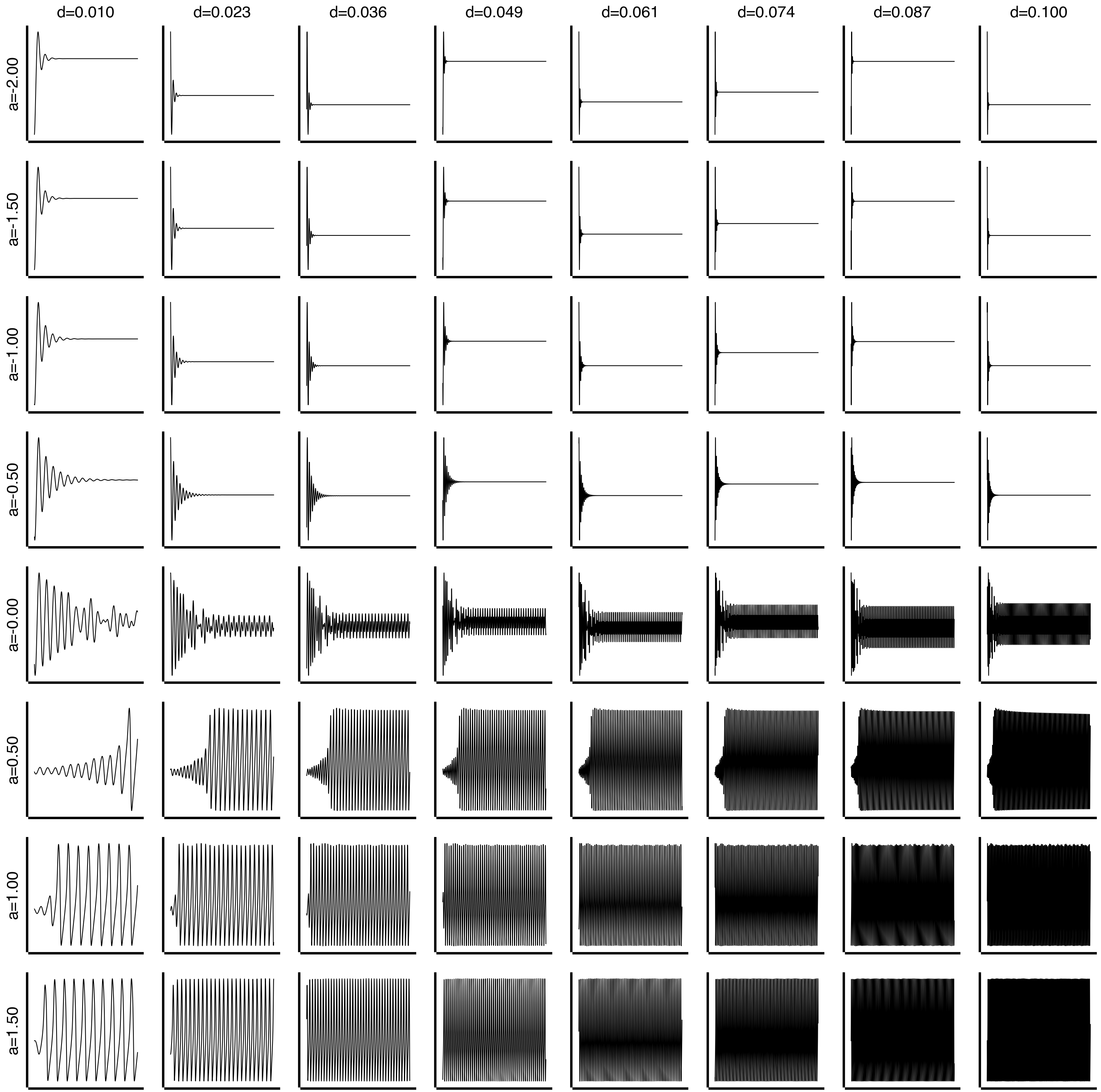
n = 8
# Explore a (controls Hopf bifurcation) and d (time scale separation)
# a ~ 0 is the bifurcation point; d controls fast/slow dynamics
state.parameters.dynamics.a = GridAxis(-2, 1.5, n)
state.parameters.dynamics.d = GridAxis(0.01, 0.1, n)
grid = Space(state, mode="product")

n_devices = jax.device_count()


def explore():
    exec = ParallelExecution(model, grid, n_pmap=n_devices, n_vmap=10)
    return exec.run()


exploration_results = explore()

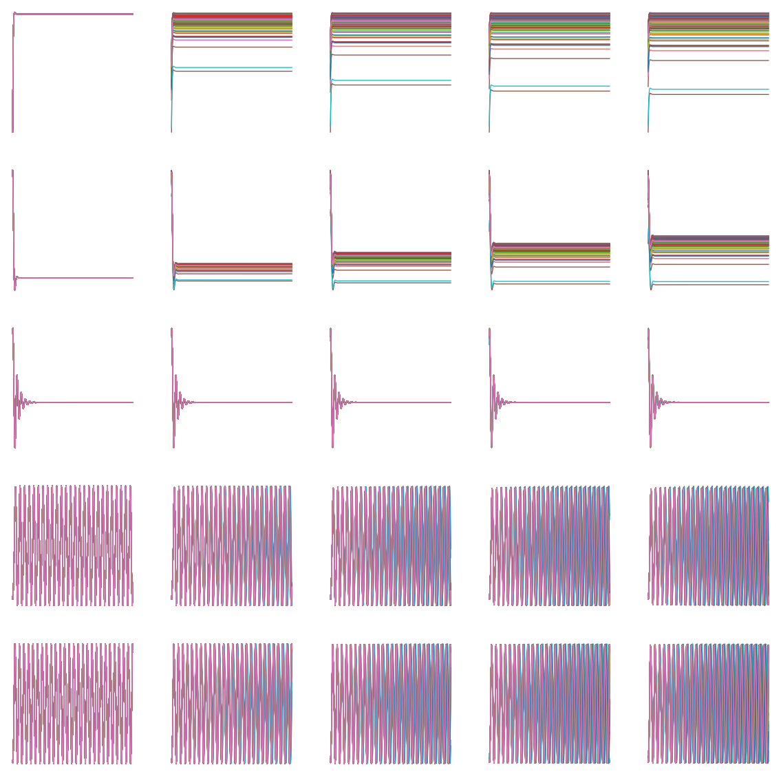
print(exploration_results.results.shape)

# Reshape: (n_pmap, n_vmap, time, state_vars, nodes, modes) -> (n_combinations, time, state_vars, nodes)
data = exploration_results.results.data.squeeze()  # remove modes dim
# Flatten n_pmap and n_vmap dimensions
data = data.reshape(-1, *data.shape[2:])  # (n_pmap*n_vmap, time, state_vars, nodes)

# Get parameter values directly from the grid (no redundant linspace!)
axis_vals = grid._generate_axis_values()
a_vals = axis_vals.parameters.dynamics.a
d_vals = axis_vals.parameters.dynamics.d

fig, axs = plt.subplots(n, n, figsize=(12, 12))
for i in range(min(n * n, data.shape[0])):
    row, col = i // n, i % n
    ax = axs[row, col]
    # data[i] has shape (time, state_vars, nodes) - plot first state variable, first node
    ax.plot(data[i, 1000:, 0, 0], linewidth=0.5)

    # Labels: rows = a (first axis), cols = d (second axis)
    if row == 0:
        ax.set_title(f"d={d_vals[col]:.3f}", fontsize=10)
    if col == 0:
        ax.set_ylabel(f"a={a_vals[row]:.2f}", fontsize=10)

bsplot.style.format_fig(fig)

for ax in fig.axes:
    ax.set_xticks([])
    ax.set_yticks([])

(8, 8, 30000, 2, 87, 1)