---
title: "Bayesian Stimulation Inference: Identifiability and Prior Sensitivity"
subtitle: "What can one noisy response tell us about stimulus strength and excitability?"
format:
html:
code-fold: false
toc: true
jupyter: python3
---
Try this notebook interactively:
[Download .ipynb](https://github.com/virtual-twin/tvboptim/blob/main/docs/workflows/Stimulation_Prior_Sensitivity.ipynb){.btn .btn-primary download="Stimulation_Prior_Sensitivity.ipynb"}
[Download .qmd](https://github.com/virtual-twin/tvboptim/blob/main/docs/workflows/Stimulation_Prior_Sensitivity.qmd){.btn .btn-secondary download="Stimulation_Prior_Sensitivity.qmd"}
[Open in Colab](https://colab.research.google.com/github/virtual-twin/tvboptim/blob/main/docs/workflows/Stimulation_Prior_Sensitivity.ipynb){.btn .btn-warning target="_blank"}
Can a recording distinguish a stronger stimulus from greater excitability?
We stimulate a single `Generic2dOscillator`, observe its fast variable $V$, and infer
the pulse amplitude $A$ and excitability parameter $I$ (`I` in the model).
We use an experiment in which their effects can compensate. We ask
which combinations the recording constrains, and how shifted prior information
can favor a different parameter explanation without substantially changing the
predicted response.
The [Basics notebook](../basics/bayesian_inference.qmd) compares posterior
sampling and variational inference. Here the focus is identifiability and prior
sensitivity. We connect three kinds of evidence: the local likelihood Fisher information,
the sampled posterior, and sensitivity to shifted informative priors. Priors on
amplitude and excitability are independent; the dependence we investigate comes
from the forward model and observation design, not an imposed prior correlation.
## 1. Define the experiment
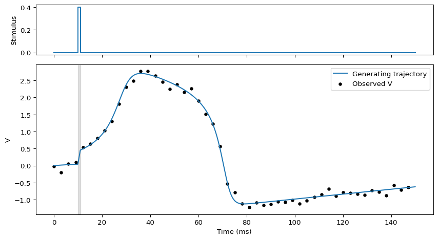
All times are in milliseconds (ms). A rectangular pulse starts at 10 ms and
lasts 1 ms. Its amplitude is unknown.
The constant drive `I`, which controls excitability in this configuration, is
also unknown. Other model coefficients and the initial state are fixed. This
is a single-region, deterministic forward model with noisy measurements of `V`;
we do not infer network connectivity or stochastic forcing.
We observe every 3 ms, beginning at the first stored solver step (0.05 ms),
over a 150 ms simulation. The observations therefore miss the
pulse itself and mainly describe the response after stimulation. Measurement
noise has known standard deviation (SD) $\sigma=0.1$, used both to generate data
and in the likelihood.
Install `tvboptim`, `numpyro`, and `matplotlib` before running the notebook.
We use the No-U-Turn Sampler (NUTS), a Hamiltonian Monte Carlo (HMC) method.
Two Markov chain Monte Carlo (MCMC) chains run sequentially on one device.
The complete notebook runs five two-chain fits, a likelihood grid, and point
optimizations, so it is more computationally demanding than the Basics example.
Initial calls also include JAX compilation. The collapsed reference comparison
runs when executing the full notebook.
```{python}
#| echo: false
#| output: false
try:
import google.colab
except ImportError:
pass
else:
import subprocess
import sys
subprocess.check_call([sys.executable, "-m", "pip", "install", "-q",
"tvboptim", "numpyro", "matplotlib"])
```
```{python}
#| code-fold: true
#| code-summary: "Imports and experiment settings"
import jax
jax.config.update("jax_enable_x64", True)

import jax.numpy as jnp
import numpy as np
import matplotlib.pyplot as plt
import numpyro
import numpyro.distributions as dist
from numpyro.infer import MCMC, NUTS
from numpyro.infer.initialization import init_to_median
from numpyro.diagnostics import summary
from IPython.display import Markdown, display

from tvboptim.experimental.network_dynamics import Network, prepare
from tvboptim.experimental.network_dynamics.dynamics.tvb import Generic2dOscillator
from tvboptim.experimental.network_dynamics.graph import DenseGraph
from tvboptim.experimental.network_dynamics.external_input import PulseInput
from tvboptim.experimental.network_dynamics.solvers import Heun

T1, DT = 150.0, 0.05
ONSET, DURATION = 10.0, 1.0
SIGMA = 0.1
TRUTH = {"amplitude": 0.4, "excitability": 0.1}
NAMES = tuple(TRUTH)
```
The input is routed to the dynamics under the name `"stimulus"`. It adds to the
`V` derivative, whereas `I` is a parameter inside the oscillator equations.
They are distinct mechanisms even when their recorded responses look similar.
See [external inputs](../network_dynamics/external_inputs.qmd) for the routing interface.
```{python}
network = Network(
    dynamics=Generic2dOscillator(
        a=-1.5, b=-15.0, c=0.0, d=0.015, e=3.0, f=1.0, tau=4.0,
        I=TRUTH["excitability"], VARIABLES_OF_INTEREST=("V",),
    ),
    coupling={},
    graph=DenseGraph(jnp.zeros((1, 1))),
    external_input={"stimulus": PulseInput(
        onset=ONSET, duration=DURATION, amplitude=TRUTH["amplitude"],
    )},
)
solve_fn, base_config = prepare(network, Heun(), t0=0.0, t1=T1, dt=DT)
times = solve_fn(base_config).ts
obs_idx = jnp.arange(0, len(times), round(3.0 / DT))
obs_times = times[obs_idx]


def trajectory(amplitude, excitability):
    config = base_config.copy()
    config.external.stimulus.amplitude = amplitude
    config.dynamics.I = excitability
    return solve_fn(config).ys[:, 0, 0]


def predict(amplitude, excitability):
    return trajectory(amplitude, excitability)[obs_idx]


clean = trajectory(**TRUTH)
observed = clean[obs_idx] + SIGMA * jax.random.normal(
    jax.random.key(42), obs_times.shape,
)
```
```{python}
#| label: fig-stim-experiment
#| fig-cap: "The known synthetic pulse and the noisy recording used for inference. The generating trajectory is available for validation only."
#| code-fold: true
#| code-summary: "Plot the stimulus and observed response"
fig, axes = plt.subplots(2, 1, figsize=(9, 5), sharex=True,
                         gridspec_kw={"height_ratios": [1, 3]})
axes[0].plot([0, ONSET, ONSET, ONSET + DURATION, ONSET + DURATION, T1],
             [0, 0, TRUTH["amplitude"], TRUTH["amplitude"], 0, 0])
axes[0].set(ylabel="Stimulus")
axes[1].plot(times, clean, label="Generating trajectory")
axes[1].scatter(obs_times, observed, color="black", s=15, label="Observed V")
axes[1].axvspan(ONSET, ONSET + DURATION, color="gray", alpha=0.25)
axes[1].set(xlabel="Time (ms)", ylabel="V")
axes[1].legend()
fig.tight_layout()
plt.show()
```
## 2. Which parameter combinations does the recording constrain?
For our independent Gaussian observations with fixed noise covariance
$\Sigma=\sigma^2\mathrm{Id}$, where $\mathrm{Id}$ is the identity matrix,
the **likelihood-only expected Fisher information** is
$$
F_\theta(\theta_0)=J_\theta(\theta_0)^\top\Sigma^{-1}J_\theta(\theta_0),
\qquad
(J_\theta)_{ij}=\frac{\partial V(t_i;\theta)}{\partial\theta_j},
\qquad \theta=(A,I).
$$
The prediction vector uses exactly the observation times in the likelihood.
This matrix describes local sensitivity of that observation distribution; it
includes no prior curvature. For this fixed-covariance Gaussian model the formula
is the expected Fisher information, not necessarily the observed negative-log-
likelihood Hessian for a particular noisy realization.
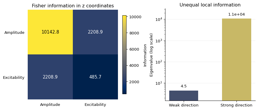
Evaluate it at the generating pair $\theta_0=(0.4,0.1)$, available here because
this is synthetic data. With real observations, evaluate at a fitted point and
check other plausible parameter values. An eigenvector with a small eigenvalue
identifies a direction in which the observation distribution changes relatively
little. It need not be an exactly flat direction.
Parameter units matter. We report eigenvalues in **dimensionless displacement
coordinates** $z=S^{-1}(\theta-\theta_0)$, with fixed scales
$S=\operatorname{diag}(0.4,0.1)$. Thus a unit displacement means an amplitude change
of 0.4 or an excitability change of 0.1. These are explicit reference scales,
not prior standard deviations. Then $F_z=S^\top F_\theta S$.
Changing these scales changes the eigenvalues, condition number, and eigenvector
angles; rank is unchanged by this invertible rescaling in exact arithmetic.
```{python}
from tvboptim.analysis import fisher_information
from tvboptim.types import Parameter

reference = jnp.array([TRUTH[name] for name in NAMES])
parameter_scales = jnp.array([0.4, 0.1])
local_parameters = {name: Parameter(TRUTH[name]) for name in NAMES}

# Parameter wrappers select leaves for this analysis; NumPyro still uses
# its own sample sites to identify the unknowns in the inference model.
raw_fisher, raw_reference, raw_labels = fisher_information(
    lambda state: predict(**state), local_parameters, sigma=SIGMA,
)
# Respect the parameter order returned by the API rather than assuming it.
order = jnp.array([raw_labels.index(name) for name in NAMES])
fisher_theta = raw_fisher[jnp.ix_(order, order)]
fisher_scaled = parameter_scales[:, None] * fisher_theta * parameter_scales[None, :]
eigenvalues, eigenvectors = jnp.linalg.eigh(fisher_scaled)
weak_direction = eigenvectors[:, 0]
strong_direction = eigenvectors[:, 1]
```
```{python}
#| label: fig-stim-fisher
#| fig-cap: "Likelihood-only Fisher information at the generating pair, in the stated dimensionless coordinates. A weak direction relative to the strong direction is different from a zero eigenvalue."
#| code-fold: true
#| code-summary: "Display the Fisher matrix, eigenvalues, and directions"
fig, axes = plt.subplots(1, 2, figsize=(9, 3.8), layout="constrained")
heatmap = axes[0].imshow(fisher_scaled, cmap="cividis")
axes[0].set(xticks=[0, 1], yticks=[0, 1], xticklabels=["Amplitude", "Excitability"],
            yticklabels=["Amplitude", "Excitability"], title="Fisher information in z coordinates")
axes[0].tick_params(length=0, pad=8)
axes[0].spines[:].set_visible(False)
for row in range(2):
    for col in range(2):
        axes[0].text(col, row, f"{fisher_scaled[row, col]:.1f}", ha="center", va="center",
                     fontsize=11,
                     color="black" if heatmap.norm(float(fisher_scaled[row, col])) > 0.55 else "white")
fig.colorbar(heatmap, ax=axes[0], shrink=0.85, label="Information")
bars = axes[1].bar(["Weak direction", "Strong direction"], eigenvalues,
                   color=plt.get_cmap("cividis")([0.25, 0.8]), width=0.55)
axes[1].set(yscale="log", ylabel="Eigenvalue (log scale)", title="Unequal local information")
axes[1].set_ylim(float(eigenvalues[0]) / 3, float(eigenvalues[-1]) * 3)
axes[1].bar_label(bars, labels=[f"{value:.2g}" for value in eigenvalues], padding=6)
axes[1].grid(axis="y", which="major", alpha=0.2)
axes[1].set_axisbelow(True)
axes[1].spines[["top", "right"]].set_visible(False)
plt.show()
print("Scaled condition number:", float(eigenvalues[-1] / eigenvalues[0]))
print("Numerical rank:", int(jnp.linalg.matrix_rank(fisher_scaled)), "of 2")
print("Weak direction (z amplitude, z excitability):", np.asarray(weak_direction))
```
Both eigenvalues are positive in this run. Their separation describes unequal
local information about parameter combinations. The weak eigenvector has opposite signs for amplitude and
excitability (its overall sign is arbitrary): increasing one can compensate for
decreasing the other.
**Structural non-identifiability** means distinct parameter values cannot be
distinguished even with ideal observations under the specified model and output.
**Practical identifiability** concerns the information available from a finite,
noisy experiment. Our analysis demonstrates a weakly constrained combination in
this experiment; an eigenvalue ratio alone does not establish that parameters
are unidentifiable to a scientifically relevant precision. See
[Gutenkunst et al. (2007)](https://doi.org/10.1371/journal.pcbi.0030189) for sensitivity
spectra and [Raue et al. (2009)](https://doi.org/10.1093/bioinformatics/btp358) for
structural and practical identifiability and profile likelihood.
### Explore the likelihood valley
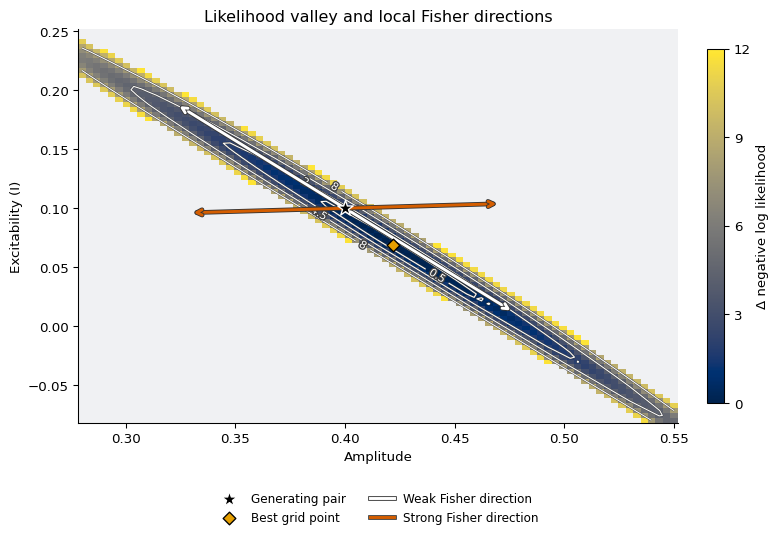
The eigenvalues summarize a local calculation. A two-dimensional exploration
makes the likelihood valley visible without adding any priors. At each grid
point, evaluate the negative log likelihood of **the actual noisy recording**,
up to its parameter-independent constant (`nll` in the code):
$$
\ell(A,I)=\frac{1}{2\sigma^2}\sum_i\left[V(t_i;A,I)-V_i^{\mathrm{obs}}\right]^2.
$$
The colors and contours below show $\Delta\ell=\ell-\min_{\mathrm{grid}}\ell$.
The minimum is over this finite grid, not a continuous maximum-likelihood fit.
Contours describe relative fit; we do not interpret them as posterior credible
regions. The same observation times and noise scale are used in inference.
```{python}
#| code-fold: true
#| code-summary: "Explore the likelihood with GridAxis, Space, and ParallelExecution"
from tvboptim.types import GridAxis, Space
from tvboptim.execution import ParallelExecution


def grid_loss(config):
    residual = (solve_fn(config).ys[obs_idx, 0, 0] - observed) / SIGMA
    return {"nll": 0.5 * jnp.sum(residual ** 2)}


grid_config = base_config.copy()
grid_config.external.stimulus.amplitude = GridAxis(0.28, 0.55, 81)
grid_config.dynamics.I = GridAxis(-0.08, 0.25, 81)
grid_space = Space(grid_config, mode="product")
grid_results = ParallelExecution(grid_loss, grid_space, n_pmap=1, n_vmap=32).run()
grid_frame = grid_results.to_dataframe()
assert len(grid_frame) == 81 * 81
assert np.isfinite(grid_frame["nll"]).all()

# Pivot using named parameter columns; do not assume execution/flattening order.
landscape = grid_frame.pivot(
    index="dynamics.I", columns="external.stimulus.amplitude", values="nll",
).sort_index().sort_index(axis=1)
amplitude_grid = landscape.columns.to_numpy(dtype=float)
excitability_grid = landscape.index.to_numpy(dtype=float)
delta_nll = landscape.to_numpy() - grid_frame["nll"].min()
best_row = grid_frame.loc[grid_frame["nll"].idxmin()]
best_grid_point = jnp.array([best_row["external.stimulus.amplitude"], best_row["dynamics.I"]])
```
```{python}
#| label: fig-stim-fisher-valley
#| fig-cap: "Likelihood exploration for the noisy recording, with Fisher directions evaluated at the generating pair. The weak direction follows the local valley; the strong direction crosses it. Light gray marks Δ negative log likelihood above 12; labeled contours are likelihood levels, not posterior credible regions. Arrow lengths are chosen for display, not uncertainty intervals."
#| code-fold: true
#| code-summary: "Overlay Fisher directions on the explored likelihood valley"
from matplotlib.lines import Line2D
import matplotlib.patheffects as path_effects

FISHER_COLORS = ("white", "#d55e00")  # Weak and strong directions, respectively.
FISHER_LINEWIDTH = 2.2
FISHER_PATH_EFFECTS = [
    path_effects.Stroke(linewidth=3.5, foreground="0.2"), path_effects.Normal()
]

fig, ax = plt.subplots(figsize=(8, 5.5), layout="constrained")
ax.set_facecolor("#f0f1f3")
display_nll = np.ma.masked_greater(delta_nll, 12)
heatmap = ax.pcolormesh(amplitude_grid, excitability_grid, display_nll,
                        shading="auto", cmap="cividis", vmin=0, vmax=12,
                        rasterized=True)
contours = ax.contour(amplitude_grid, excitability_grid, delta_nll,
                      levels=[0.5, 2.0, 4.5, 8.0], colors="white", linewidths=0.8)
contours.set_path_effects([path_effects.withStroke(linewidth=1.5, foreground="0.25")])
contour_labels = ax.clabel(contours, inline=True, fontsize=8, fmt="%g")
for text in contour_labels:
    text.set_path_effects([path_effects.withStroke(linewidth=2, foreground="0.25")])
for direction, length, color in zip(
    (weak_direction, strong_direction), (0.9, 0.18), FISHER_COLORS,
):
    # Eigenvectors were computed in z coordinates: map displacements back to (A, I).
    offset = length * parameter_scales * direction
    arrow = ax.annotate("", xy=reference + offset, xytext=reference - offset,
                        arrowprops=dict(arrowstyle="<->", color=color, lw=FISHER_LINEWIDTH), zorder=4)
    arrow.arrow_patch.set_path_effects(FISHER_PATH_EFFECTS)
ax.scatter(*reference, color="black", edgecolor="white", marker="*", s=150,
            label="Generating pair", zorder=5)
ax.scatter(*best_grid_point, color="#e69f00", edgecolor="black", marker="D", s=45,
            label="Best grid point", zorder=5)
handles, labels = ax.get_legend_handles_labels()
fisher_handles = [
    Line2D([0], [0], color=color, lw=FISHER_LINEWIDTH, path_effects=FISHER_PATH_EFFECTS)
    for color in FISHER_COLORS
]
handles += fisher_handles
labels += ["Weak Fisher direction", "Strong Fisher direction"]
ax.legend(handles, labels, loc="upper center", bbox_to_anchor=(0.5, -0.15),
          ncol=2, frameon=False, fontsize=9)
ax.set(xlabel="Amplitude", ylabel="Excitability (I)", title="Likelihood valley and local Fisher directions")
ax.spines[["top", "right"]].set_visible(False)
fig.colorbar(heatmap, ax=ax, label="Δ negative log likelihood", ticks=[0, 3, 6, 9, 12],
             shrink=0.9, pad=0.03)
plt.show()
```
The arrows are transformed back from the stated dimensionless coordinates, so
they need not look perpendicular on these physical axes. Their origin is the
generating pair, whereas the grid minimum can move because the recording is noisy.
The weak direction should follow the valley locally; a straight arrow need not
follow it farther away. This grid checks the shape only in the displayed region.
Next we compare the weak Fisher direction with the posterior explored by NUTS.
Neither this local calculation nor successful sampler diagnostics establishes
global uniqueness.
## 3. Infer both parameters and compare with the local geometry
Our baseline assumptions are a positive amplitude with a log-normal prior
(median 0.4, log-scale standard deviation 0.6), and excitability with a Normal
prior (mean 0.1, standard deviation 0.15). Negative `I` is allowed: this is a
signed drive in the model. These moderately broad priors still carry information.
The prior centers happen to equal the generating values in this controlled
example. That is a favorable synthetic setup, not knowledge obtained from the
recording. Later we shift the center of one informative prior at a time to test
how a biased or conflicting information source changes the inferred explanation.
Truth-centered informative priors remain as a small reference comparison.
```{python}
AMP_MEDIAN, EXC_MEAN = 0.4, 0.1
BASE_AMP_SCALE, BASE_EXC_SCALE = 0.6, 0.15


def model(data=None, amp_scale=BASE_AMP_SCALE, exc_scale=BASE_EXC_SCALE,
          amp_median=AMP_MEDIAN, exc_mean=EXC_MEAN):
    amplitude = numpyro.sample("amplitude", dist.LogNormal(jnp.log(amp_median), amp_scale))
    excitability = numpyro.sample("excitability", dist.Normal(exc_mean, exc_scale))
    numpyro.sample(
        "obs", dist.Normal(predict(amplitude, excitability), SIGMA).to_event(1), obs=data,
    )
```
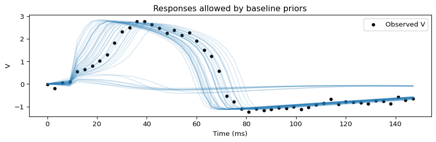
Before sampling the posterior, inspect noiseless trajectories from baseline prior
draws. Their spread shows the response uncertainty before conditioning on the
recording. This finite sample checks part of the prior support.
```{python}
#| code-fold: true
#| code-summary: "Inspect trajectories from the baseline priors"
keys = jax.random.split(jax.random.key(1), 2)
prior_amplitude = dist.LogNormal(jnp.log(AMP_MEDIAN), BASE_AMP_SCALE).sample(keys[0], (40,))
prior_excitability = dist.Normal(EXC_MEAN, BASE_EXC_SCALE).sample(keys[1], (40,))
prior_responses = jax.jit(jax.vmap(predict))(prior_amplitude, prior_excitability)
assert bool(jnp.all(jnp.isfinite(prior_responses)))
fig, ax = plt.subplots(figsize=(9, 3))
ax.plot(obs_times, prior_responses.T, color="tab:blue", alpha=0.15)
ax.scatter(obs_times, observed, color="black", s=15, label="Observed V")
ax.set(xlabel="Time (ms)", ylabel="V", title="Responses allowed by baseline priors")
ax.legend()
fig.tight_layout()
plt.show()
```
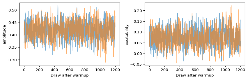
Use two chains and retain their separation for diagnostics. A full mass matrix
helps NUTS handle parameter dependence. For the baseline fit, initialize each
chain using medians of random prior draws. Broad default initialization can place
this nonlinear oscillator in a poorly fitting region where a chain gets stuck.
Check divergences, effective sample size (ESS), and $\hat R$ (R-hat), which
compares variation within and between chains. A divergence flags excessive
numerical error along a Hamiltonian trajectory and can indicate poor posterior
exploration. The runner requires no divergences, R-hat at most 1.01, and ESS of
at least 200 for each inferred parameter. These thresholds screen for sampling
problems; they do not prove convergence or ensure sufficient precision for every
posterior summary. See the [Basics sampling discussion](../basics/bayesian_inference.qmd#sample-with-hamiltonian-monte-carlo-hmc)
for diagnostic interpretation.
```{python}
def fit(seed, amp_scale, exc_scale, amp_median=AMP_MEDIAN, exc_mean=EXC_MEAN,
        init_params=None):
    sampler = MCMC(
        NUTS(model, dense_mass=True, target_accept_prob=0.9,
             init_strategy=init_to_median(num_samples=25)),
        num_warmup=700, num_samples=1200, num_chains=2,
        chain_method="sequential", progress_bar=False,
    )
    sampler.run(jax.random.key(seed), data=observed, init_params=init_params,
                amp_scale=amp_scale, exc_scale=exc_scale,
                amp_median=amp_median, exc_mean=exc_mean)
    stats = summary(sampler.get_samples(group_by_chain=True), group_by_chain=True)
    divergences = int(sampler.get_extra_fields()["diverging"].sum())
    rhats = np.array([stats[name]["r_hat"] for name in NAMES])
    effective_sizes = np.array([stats[name]["n_eff"] for name in NAMES])
    if (divergences or not np.all(np.isfinite(rhats)) or not np.all(np.isfinite(effective_sizes))
            or rhats.max() > 1.01 or effective_sizes.min() < 200):
        raise RuntimeError(
            f"Sampling checks failed: {divergences} divergences, "
            f"max R-hat={rhats.max():.3f}, min ESS={effective_sizes.min():.0f}. "
            "Investigate initialization, geometry, and sampling settings before interpreting this fit."
        )
    return sampler


baseline = fit(10, BASE_AMP_SCALE, BASE_EXC_SCALE)
baseline.print_summary()
baseline_samples = baseline.get_samples()
```
Read the effective sample sizes and $\hat R$ alongside the divergence count.
Inspect traces for chains getting stuck in different regions. If diagnostics
are poor, resolve the sampling problem before interpreting the intervals.
```{python}
#| code-fold: true
#| code-summary: "Inspect baseline chain traces"
fig, axes = plt.subplots(1, 2, figsize=(9, 3))
chains = baseline.get_samples(group_by_chain=True)
for ax, name in zip(axes, NAMES):
    ax.plot(chains[name].T, alpha=0.6)
    ax.set(xlabel="Draw after warmup", ylabel=name)
fig.tight_layout()
plt.show()
```
```{python}
#| code-fold: true
#| code-summary: "Plot the joint posterior and marginal distributions"
fig, axes = plt.subplots(1, 3, figsize=(12, 3.3))
axes[0].scatter(baseline_samples["amplitude"], baseline_samples["excitability"],
                s=5, alpha=0.2)
axes[0].scatter(TRUTH["amplitude"], TRUTH["excitability"], marker="*", s=100,
                color="black", label="Generating pair")
axes[0].set(xlabel="Amplitude", ylabel="Excitability (I)")
axes[0].legend()
for ax, name in zip(axes[1:], NAMES):
    ax.hist(baseline_samples[name], bins=35, density=True, alpha=0.6)
    ax.axvline(TRUTH[name], color="black")
    ax.set(xlabel=name, ylabel="Posterior density")
fig.tight_layout()
plt.show()
print("Posterior correlation:", float(jnp.corrcoef(
    baseline_samples["amplitude"], baseline_samples["excitability"])[0, 1]))
```
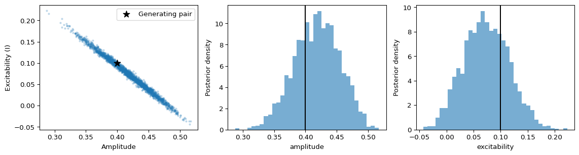
The joint cloud shows a trade-off: a stronger pulse can be accompanied by a lower
excitability value. The recording constrains combinations of parameters more
strongly than either parameter separately. A point estimate alone hides this
dependence.
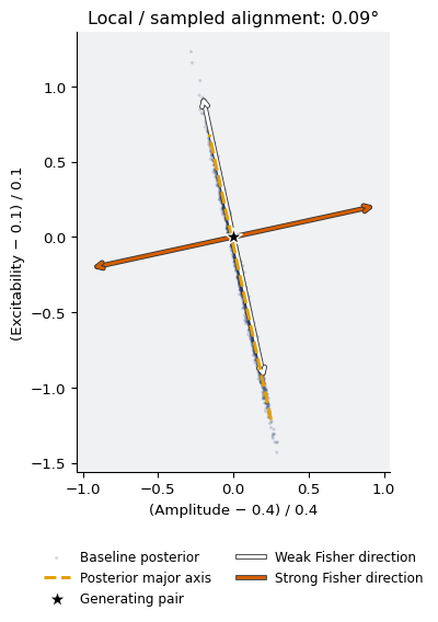
Compare the sampled dependence with the Fisher prediction in **the same scaled
coordinates**. The posterior's major covariance eigenvector is a summary of its
sampled spread. We compute its angle to the weak Fisher direction rather than
assuming alignment. The lines below indicate orientation only; they are not
credible intervals or a Fisher-based approximation to the full posterior.
```{python}
posterior_z = (jnp.column_stack([baseline_samples[name] for name in NAMES])
               - reference) / parameter_scales
posterior_covariance = jnp.cov(posterior_z.T)
_, posterior_axes = jnp.linalg.eigh(posterior_covariance)
posterior_major = posterior_axes[:, -1]
alignment = jnp.clip(jnp.abs(jnp.dot(weak_direction, posterior_major)), 0.0, 1.0)
alignment_angle = jnp.degrees(jnp.arccos(alignment))
print(f"Angle between weak Fisher direction and posterior major axis: {alignment_angle:.2f}°")
```
```{python}
#| label: fig-stim-fisher-posterior
#| fig-cap: "Baseline posterior in dimensionless coordinates, with local Fisher arrows through the generating point and the sampled major axis through the posterior mean. Fisher arrows use the same colors and styling as the likelihood exploration. All lengths are chosen for display."
#| code-fold: true
#| code-summary: "Overlay Fisher directions and the posterior major axis"
fig, ax = plt.subplots(figsize=(6.5, 5.8), layout="constrained")
ax.set_facecolor("#f0f1f3")
ax.scatter(posterior_z[:, 0], posterior_z[:, 1], s=5, alpha=0.2,
           color=plt.get_cmap("cividis")(0.15), edgecolors="none",
           label="Baseline posterior", rasterized=True)
line_extent = float(jnp.quantile(jnp.linalg.norm(posterior_z, axis=1), 0.95))
for direction, color in zip((weak_direction, strong_direction), FISHER_COLORS):
    offset = line_extent * direction
    arrow = ax.annotate("", xy=offset, xytext=-offset,
                        arrowprops=dict(arrowstyle="<->", color=color, lw=FISHER_LINEWIDTH), zorder=4)
    arrow.arrow_patch.set_path_effects(FISHER_PATH_EFFECTS)
    ax.update_datalim(np.asarray(jnp.stack((-offset, offset))))
segment = posterior_z.mean(axis=0) + jnp.array([-line_extent, line_extent])[:, None] * posterior_major
ax.plot(segment[:, 0], segment[:, 1], "--", color="#e69f00", lw=2.2,
        label="Posterior major axis", zorder=5)
ax.scatter(0, 0, marker="*", s=150, color="black", edgecolor="white",
           label="Generating pair", zorder=6)
ax.set(xlabel="(Amplitude − 0.4) / 0.4", ylabel="(Excitability − 0.1) / 0.1",
       title=f"Local / sampled alignment: {alignment_angle:.2f}°", aspect="equal")
handles, labels = ax.get_legend_handles_labels()
handles += fisher_handles
labels += ["Weak Fisher direction", "Strong Fisher direction"]
ax.legend(handles, labels, loc="upper center", bbox_to_anchor=(0.5, -0.15),
          ncol=2, frameon=False, fontsize=9)
ax.spines[["top", "right"]].set_visible(False)
plt.show()
```
Close alignment supports a common explanation for the two results: the likelihood
changes relatively little along the direction explored by the elongated posterior.
The Fisher matrix is evaluated at one point and excludes priors, while the
posterior includes priors and nonlinear behavior across its sampled region.
They need not agree in a different experiment or with stronger priors.
### Different parameters, similar recorded responses
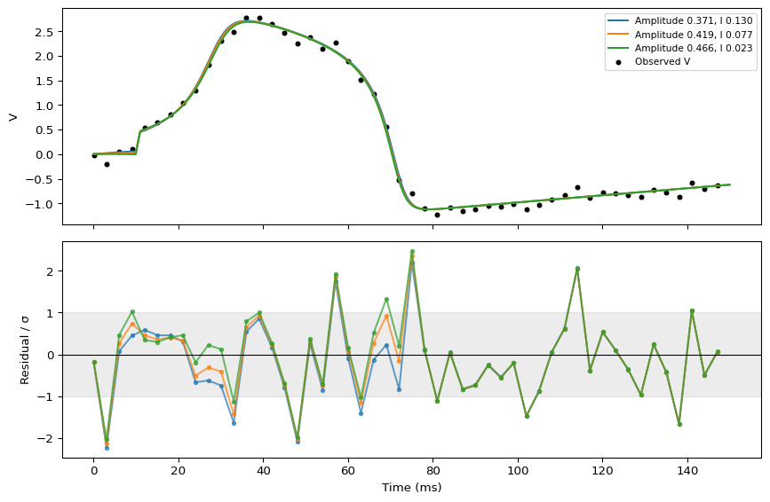
Choose actual joint posterior draws near the 10th, 50th, and 90th amplitude
percentiles. Keep each draw's matching excitability value: independently pairing
marginal quantiles can create a combination unsupported by the posterior.
These are illustrative draws, not a credible band or a set of alternative optima.
```{python}
levels = jnp.array([0.1, 0.5, 0.9])
targets = jnp.quantile(baseline_samples["amplitude"], levels)
selected = jnp.argmin(jnp.abs(baseline_samples["amplitude"][:, None] - targets), axis=0)
representatives = {name: baseline_samples[name][selected] for name in NAMES}
representative_curves = jax.jit(jax.vmap(trajectory))(**representatives)
```
```{python}
#| label: fig-stim-tradeoff
#| fig-cap: "Three joint posterior draws. Residuals at the measurement times are shown in units of the observation noise; the shaded range is ±1 noise standard deviation, not a posterior interval."
#| code-fold: true
#| code-summary: "Compare representative responses and their residuals"
fig, axes = plt.subplots(2, 1, figsize=(9, 6), sharex=True)
for i, curve in enumerate(representative_curves):
    label = (f"Amplitude {representatives['amplitude'][i]:.3f}, "
             f"I {representatives['excitability'][i]:.3f}")
    axes[0].plot(times, curve, label=label)
    axes[1].plot(obs_times, (observed - curve[obs_idx]) / SIGMA, ".-", alpha=0.7)
axes[0].scatter(obs_times, observed, s=12, color="black", label="Observed V")
axes[0].set(ylabel="V")
axes[0].legend(fontsize=8)
axes[1].axhspan(-1, 1, color="gray", alpha=0.15)
axes[1].axhline(0, color="black", lw=0.8)
axes[1].set(xlabel="Time (ms)", ylabel="Residual / σ")
fig.tight_layout()
plt.show()
```
The trajectories differ, but those differences are small relative to the
measurement noise at the recorded times.
::: {.callout-note collapse="true"}
## Check the numerical time step
The posterior depends on the numerical forward model. Halve the integration step
at the three representative parameter pairs and compare predictions at the same
measurement times. This local check is especially relevant for a rectangular
pulse with discontinuities. It does not replace refitting at a finer resolution
when numerical changes are appreciable.
```{python}
#| code-fold: true
#| code-summary: "Compare predictions after halving the time step"
fine_solve, fine_config = prepare(network, Heun(), t0=0.0, t1=T1, dt=DT / 2)
fine_times = fine_solve(fine_config).ts
# Match timestamps explicitly: both solvers save after their first step,
# so doubling array indices would compare different physical times.
fine_idx = jnp.argmin(jnp.abs(fine_times[:, None] - obs_times[None, :]), axis=0)
np.testing.assert_allclose(fine_times[fine_idx], obs_times, atol=1e-10, rtol=0)
numerical_rows = [
    "| Amplitude | Excitability | Max prediction change / σ | Change in log likelihood |",
    "|--:|--:|--:|--:|",
]
for i in range(3):
    config = fine_config.copy()
    config.external.stimulus.amplitude = representatives["amplitude"][i]
    config.dynamics.I = representatives["excitability"][i]
    refined = fine_solve(config).ys[fine_idx, 0, 0]
    original = representative_curves[i, obs_idx]
    change = float(jnp.max(jnp.abs(refined - original)) / SIGMA)
    delta_log_likelihood = float(jnp.sum(
        dist.Normal(refined, SIGMA).log_prob(observed)
        - dist.Normal(original, SIGMA).log_prob(observed)
    ))
    numerical_rows.append(
        f"| {representatives['amplitude'][i]:.3f} | {representatives['excitability'][i]:.3f} "
        f"| {change:.3f} | {delta_log_likelihood:.3f} |"
    )
display(Markdown("\n".join(numerical_rows)))
```
:::
## 4. Shift informative priors along the trade-off
Suppose a stimulator calibration suggests a lower amplitude, or an independent
assay suggests lower excitability. We deliberately shift one informative prior
below the generating value while leaving the other prior unchanged. The negative
parameter dependence suggests that the *other* parameter will move upward to
compensate. This is a prediction to check, not a constraint imposed on the sampler.
| Scenario | Amplitude prior: median, log-scale SD | Excitability prior: mean, SD |
|:--|:--|:--|
| Baseline | 0.4, 0.6 | 0.1, 0.15 |
| Lower amplitude prior | **0.32, 0.04** | 0.1, 0.15 |
| Lower excitability prior | 0.4, 0.6 | **0.0, 0.025** |
These are hypothetical, deliberately biased information sources in a synthetic
experiment. We do not infer their reliability or compare posterior probabilities
of mechanisms. A real assay needs a justified mapping to the model's `I`, and a
prior derived from the same recording would count that evidence twice.
For these sensitivity fits, initialize the two chains at different joint draws
from the successful baseline fit, near its 10th and 90th amplitude percentiles.
Independent prior-based starts can land in poorly fitting response regimes of
this nonlinear model and fail to mix. Each scenario gets fresh warmup and targets
its own posterior; the baseline draws supply starting locations only, not an
extra prior or likelihood contribution. This strategy explores the known response
region and does not establish the absence of disconnected posterior modes.
```{python}
# NumPyro's explicit init_params use unconstrained coordinates: log amplitude
# for the positive sample site, and unchanged excitability for the real site.
start_targets = jnp.quantile(baseline_samples["amplitude"], jnp.array([0.1, 0.9]))
start_idx = jnp.argmin(jnp.abs(baseline_samples["amplitude"][:, None] - start_targets), axis=0)
scenario_initials = {
    "amplitude": jnp.log(baseline_samples["amplitude"][start_idx]),
    "excitability": baseline_samples["excitability"][start_idx],
}
scenarios = {
    "Baseline": dict(amp_scale=BASE_AMP_SCALE, exc_scale=BASE_EXC_SCALE),
    "Lower amplitude prior": dict(amp_median=0.32, amp_scale=0.04, exc_scale=BASE_EXC_SCALE),
    "Lower excitability prior": dict(exc_mean=0.0, amp_scale=BASE_AMP_SCALE, exc_scale=0.025),
}
fits = {"Baseline": baseline}
for seed, (label, settings) in enumerate(list(scenarios.items())[1:], start=11):
    fits[label] = fit(seed, init_params=scenario_initials, **settings)
posteriors = {label: sampler.get_samples() for label, sampler in fits.items()}
```
The following diagnostics cover **every scenario**, not just the baseline.
The credible intervals below are 5th–95th percentiles: 90% marginal posterior
intervals, conditional on that scenario's assumptions. They do not form a joint
90% region. Comparisons across scenarios describe prior sensitivity, not posterior
probabilities of competing mechanisms.
```{python}
#| code-fold: true
#| code-summary: "Display diagnostics and parameter credible intervals"
diagnostic_rows = [
    "| Scenario | Divergences | Max R-hat | Min effective sample size |",
    "|:--|--:|--:|--:|",
]
interval_rows = [
    "| Scenario | Parameter | Median | 90% credible interval |",
    "|:--|:--|--:|:--|",
]
for label, sampler in fits.items():
    stats = summary(sampler.get_samples(group_by_chain=True), group_by_chain=True)
    divergences = int(sampler.get_extra_fields()["diverging"].sum())
    max_rhat = max(float(stats[name]["r_hat"]) for name in NAMES)
    min_ess = min(float(stats[name]["n_eff"]) for name in NAMES)
    diagnostic_rows.append(f"| {label} | {divergences} | {max_rhat:.3f} | {min_ess:.0f} |")
    for name in NAMES:
        lo, median, hi = jnp.quantile(posteriors[label][name], jnp.array([0.05, 0.5, 0.95]))
        interval_rows.append(f"| {label} | {name} | {median:.3f} | [{lo:.3f}, {hi:.3f}] |")
display(Markdown("\n".join(diagnostic_rows)))
display(Markdown("\n".join(interval_rows)))
```
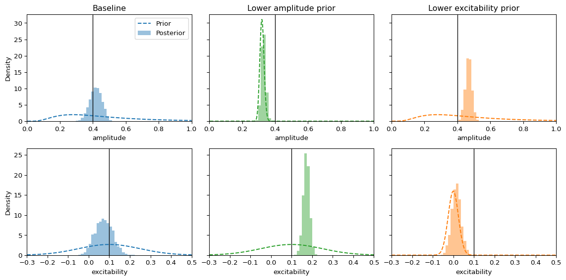
Compare priors and posteriors on the same horizontal ranges. The parameter whose
prior was left unchanged can move into a different region because the likelihood
couples it to the directly constrained parameter. A narrow posterior can therefore
be both precise and displaced from the generating values. It is conditional on
the assumed information source, not evidence that this source is correct.
```{python}
#| label: fig-stim-prior-sensitivity
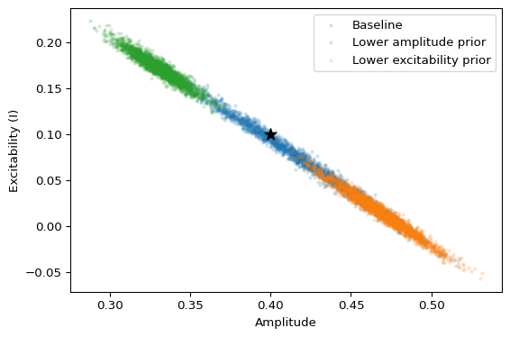
#| fig-cap: "Columns use identical observations and likelihoods. Dashed densities are priors; filled histograms are marginal posteriors. Black vertical lines mark generating values. Axis ranges are shared across scenarios for each parameter."
#| code-fold: true
#| code-summary: "Compare scenario priors, marginals, and joint posteriors"
colors = ("tab:blue", "tab:green", "tab:orange")
grids = {"amplitude": jnp.linspace(0.0, 1.0, 400),
         "excitability": jnp.linspace(-0.3, 0.5, 400)}
fig, axes = plt.subplots(2, 3, figsize=(12, 6), sharex="row", sharey="row")
for col, ((label, settings), color) in enumerate(zip(scenarios.items(), colors)):
    priors = {
        "amplitude": dist.LogNormal(jnp.log(settings.get("amp_median", AMP_MEDIAN)), settings["amp_scale"]),
        "excitability": dist.Normal(settings.get("exc_mean", EXC_MEAN), settings["exc_scale"]),
    }
    for row, name in enumerate(NAMES):
        ax = axes[row, col]
        grid = grids[name]
        ax.plot(grid, jnp.exp(priors[name].log_prob(grid)), color=color, ls="--", label="Prior")
        ax.hist(posteriors[label][name], bins=np.linspace(float(grid[0]), float(grid[-1]), 65),
                density=True, color=color, alpha=0.45, label="Posterior")
        ax.axvline(TRUTH[name], color="black", lw=1)
        ax.set(xlabel=name, xlim=(float(grid[0]), float(grid[-1])))
        if row == 0:
            ax.set_title(label)
        if col == 0:
            ax.set_ylabel("Density")
axes[0, 0].legend()
fig.tight_layout()
plt.show()

fig, ax = plt.subplots(figsize=(6, 4))
for (label, samples), color in zip(posteriors.items(), colors):
    ax.scatter(samples["amplitude"], samples["excitability"], s=5, alpha=0.15,
                color=color, label=label)
ax.scatter(TRUTH["amplitude"], TRUTH["excitability"], color="black", marker="*", s=100)
ax.set(xlabel="Amplitude", ylabel="Excitability (I)")
ax.legend()
fig.tight_layout()
plt.show()
```
The shifted priors move the posterior along the trade-off. Section 5 checks
whether these parameter explanations still account for the recording; larger
or incompatible prior shifts could compromise the fit.
::: {.callout-note collapse="true"}
## Reference: tighter priors without a shift
To separate the effect of tightening from the effect of shifting, repeat with the
same informative widths centered on the generating values. These two fits are
reference controls for the synthetic experiment, not additional evidence. Their
diagnostics and marginal equal-tailed 90% credible intervals are reported
alongside the same-width shifted fits.
```{python}
#| code-fold: true
#| code-summary: "Fit truth-centered reference priors and compare intervals"
reference_settings = {
    "Amplitude centered": dict(amp_scale=0.04, exc_scale=BASE_EXC_SCALE),
    "Excitability centered": dict(amp_scale=BASE_AMP_SCALE, exc_scale=0.025),
}
reference_fits = {
    label: fit(seed, init_params=scenario_initials, **settings)
    for seed, (label, settings) in enumerate(reference_settings.items(), start=13)
}
reference_rows = [
    "| Scenario | Divergences | Max R-hat | Min ESS | Amplitude: median [90% interval] | Excitability: median [90% interval] |",
    "|:--|--:|--:|--:|:--|:--|",
]
for label, sampler in {**reference_fits, **{k: v for k, v in fits.items() if k != "Baseline"}}.items():
    draws = sampler.get_samples()
    stats = summary(sampler.get_samples(group_by_chain=True), group_by_chain=True)
    intervals = []
    for name in NAMES:
        lo, median, hi = jnp.quantile(draws[name], jnp.array([0.05, 0.5, 0.95]))
        intervals.append(f"{median:.3f} [{lo:.3f}, {hi:.3f}]")
    reference_rows.append(
        f"| {label} | {int(sampler.get_extra_fields()['diverging'].sum())} "
        f"| {max(float(stats[n]['r_hat']) for n in NAMES):.3f} "
        f"| {min(float(stats[n]['n_eff']) for n in NAMES):.0f} | {' | '.join(intervals)} |"
    )
display(Markdown("\n".join(reference_rows)))
```
Comparing each centered fit to its shifted counterpart isolates the effect
of the prior center.
:::
### Maximum a posteriori (MAP) estimation
Drawing optimizer starting points from a prior **does not include that prior in
the objective**. With our fixed Gaussian noise, minimizing mean squared error
(MSE) gives maximum likelihood estimation (MLE). Agreement of likelihood optima
from different starts reflects their common objective, not insensitivity to priors.
MAP estimation incorporates the prior throughout optimization:
$$
\hat\theta_{\mathrm{MAP}}
=\arg\max_\theta p(\theta\mid V^{\mathrm{obs}})
=\arg\min_\theta\left[-\log p(V^{\mathrm{obs}}\mid\theta)-\log p(\theta)\right].
$$
The evidence is constant with respect to $\theta$, so it is unnecessary for this
optimization. The prior contributes to the objective throughout fitting, acting
as a penalty on less plausible values. A Gaussian prior, for example, contributes
a squared deviation scaled by its variance. With a flat prior over the allowed
region, MAP and MLE have the same objective up to a constant.
| Calculation | Objective or target | What it reports |
|:--|:--|:--|
| MLE / least squares | Likelihood only | A best-fitting point |
| MAP in stated parameter coordinates | Likelihood × prior | A posterior mode, which can shift with the prior |
| Posterior inference | Likelihood × prior | A distribution over plausible parameter combinations |
A density mode can change under nonlinear reparameterization, so MAP coordinates
must be stated.
NumPyro supports MAP directly through
[`AutoDelta`](https://num.pyro.ai/en/stable/autoguide.html#autodelta), a guide with
all its probability mass at a learned point. We use the **same model and scenario
arguments as NUTS**. `AutoDelta` targets the density mode in the original,
constrained sample-site coordinates: here positive amplitude and real excitability.
Although positivity is enforced internally through a transform, this is not the
mode of the posterior density expressed in log amplitude.
We fit this guide through NumPyro's stochastic variational inference (SVI)
interface. `Trace_ELBO` supplies the evidence lower bound (ELBO) objective;
with `AutoDelta` in this model, minimizing its negative amounts to minimizing
the negative log joint density. The check below verifies this equality.
[`Minimize`](https://num.pyro.ai/en/stable/optimizers.html#minimize) uses the
Broyden–Fletcher–Goldfarb–Shanno (BFGS) gradient-based optimizer. One SVI update
runs up to 200 internal BFGS iterations. `guide.median` returns the fitted point
of the delta distribution, not the median of the sampled posterior.
```{python}
from numpyro.infer import SVI, Trace_ELBO
from numpyro.infer.autoguide import AutoDelta
from numpyro.infer.initialization import init_to_value
from numpyro.optim import Minimize


def fit_map(start, settings, seed):
    guide = AutoDelta(model, init_loc_fn=init_to_value(values=start))
    svi = SVI(model, guide,
              Minimize(method="BFGS", options={"maxiter": 200, "gtol": 1e-7}),
              Trace_ELBO())
    result = svi.run(jax.random.key(seed), 1, data=observed,
                     progress_bar=False, **settings)
    return guide.median(result.params), svi.evaluate(result.state, data=observed, **settings)
```
Use two distinct, well-fitting baseline draws as starting points, as in the
sensitivity sampling runs. For every scenario we check that both fits reduce
their own objective, have small gradients, and agree on the fitted point. These
checks establish agreement of local solutions from these starts, not a guarantee
of finding a global mode.
```{python}
#| code-fold: true
#| code-summary: "Fit and check MAP estimates from two starting points"
from numpyro.infer.util import log_density

map_starts = [{name: baseline_samples[name][start_idx[i]] for name in NAMES} for i in range(2)]
map_points = {}
map_rows = [
    "| Scenario | MAP amplitude | MAP excitability | Largest scaled gradient norm | Scaled distance between fits |",
    "|:--|--:|--:|--:|--:|",
]
for scenario_index, (label, settings) in enumerate(scenarios.items()):
    # Use the same dimensionless coordinates as in the Fisher analysis for
    # reporting gradient sizes and distances. This only re-expresses the
    # objective; it does not add a density-transformation Jacobian.
    def negative_log_joint(z):
        theta = reference + parameter_scales * z
        return -log_density(model, (), dict(data=observed, **settings), dict(zip(NAMES, theta)))[0]

    solutions, gradient_norms = [], []
    for i, start in enumerate(map_starts):
        point, svi_objective = fit_map(start, settings, 50 + 2 * scenario_index + i)
        theta = jnp.array([point[name] for name in NAMES])
        z = (theta - reference) / parameter_scales
        z_start = (jnp.array([start[name] for name in NAMES]) - reference) / parameter_scales
        value, gradient = jax.value_and_grad(negative_log_joint)(z)
        gradient_norm = float(jnp.linalg.norm(gradient, ord=jnp.inf))
        np.testing.assert_allclose(svi_objective, value, rtol=0, atol=1e-6)
        assert bool(jnp.isfinite(value)) and gradient_norm < 1e-4
        assert float(value) <= float(negative_log_joint(z_start)) + 1e-6
        solutions.append(theta)
        gradient_norms.append(gradient_norm)
    distance = float(jnp.linalg.norm((solutions[0] - solutions[1]) / parameter_scales))
    assert distance < 1e-4
    map_points[label] = solutions[0]
    map_rows.append(
        f"| {label} | {solutions[0][0]:.3f} | {solutions[0][1]:.3f} "
        f"| {max(gradient_norms):.2e} | {distance:.2e} |"
    )
display(Markdown("\n".join(map_rows)))
```
```{python}
#| label: fig-stim-map-posterior
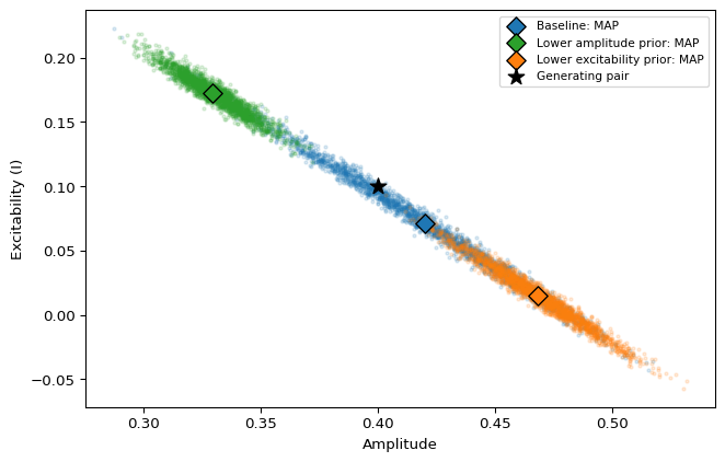
#| fig-cap: "MAP points and NUTS draws target the same model under each prior scenario. The points move with the priors, but do not show the width or dependence of the surrounding distributions. The generating pair is marked separately."
#| code-fold: true
#| code-summary: "Overlay MAP estimates on the sampled posteriors"
fig, ax = plt.subplots(figsize=(7, 4.5))
for (label, samples), color in zip(posteriors.items(), colors):
    ax.scatter(samples["amplitude"], samples["excitability"], s=5, alpha=0.15, color=color)
    ax.scatter(*map_points[label], marker="D", s=85, color=color, edgecolor="black",
                zorder=5, label=f"{label}: MAP")
ax.scatter(*reference, color="black", marker="*", s=130, zorder=6, label="Generating pair")
ax.set(xlabel="Amplitude", ylabel="Excitability (I)")
ax.legend(fontsize=8)
fig.tight_layout()
plt.show()
```
The shifted priors move both the MAP points and the posterior clouds. The NUTS
draws also show the remaining spread and parameter dependence. A MAP point alone
provides no uncertainty interval, and a histogram of multi-start optimization
endpoints is not a posterior distribution. The distinction is between a point
estimate and a distribution: both optimization and NUTS use gradients here.
## 5. Check predictions and interpret the limits
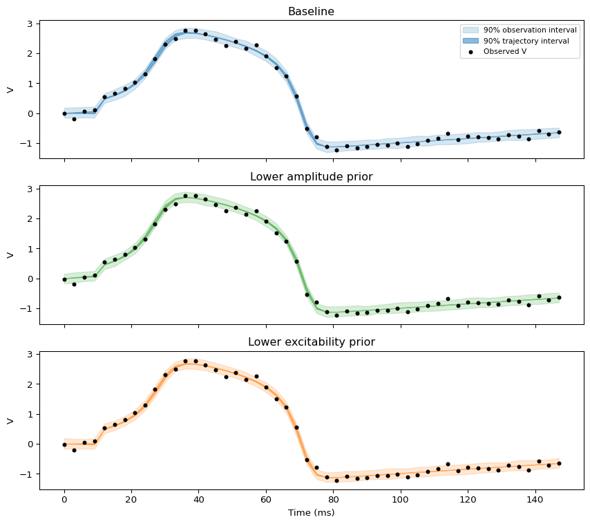
Generate new responses from posterior parameter draws. The **trajectory interval**
reflects parameter uncertainty; the **observation interval** additionally includes
measurement noise. We use draws from both chains and keep complete parameter pairs.
Intervals are pointwise 90% intervals at the recorded times, not simultaneous
bands over the entire response.
```{python}
predictions = {}
for seed, (label, samples) in enumerate(posteriors.items(), start=20):
    # Evenly spaced draws span both sequential chains.
    take = jnp.linspace(0, len(samples["amplitude"]) - 1, 300).astype(int)
    response = jax.jit(jax.vmap(predict))(**{name: samples[name][take] for name in NAMES})
    new_observation = response + SIGMA * jax.random.normal(jax.random.key(seed), response.shape)
    predictions[label] = {"trajectory": response, "observation": new_observation}
```
```{python}
#| label: fig-stim-predictive
#| fig-cap: "Shifted priors can change the inferred parameter explanation while predictions of the already observed response remain similar. Both interval types are computed at observation times; connecting them is a visual aid."
#| code-fold: true
#| code-summary: "Plot trajectory and observation intervals for each scenario"
fig, axes = plt.subplots(3, 1, figsize=(9, 8), sharex=True, sharey=True)
for ax, (label, prediction), color in zip(axes, predictions.items(), colors):
    for site, alpha in (("observation", 0.18), ("trajectory", 0.5)):
        lo, hi = jnp.quantile(prediction[site], jnp.array([0.05, 0.95]), axis=0)
        ax.fill_between(obs_times, lo, hi, color=color, alpha=alpha,
                         label=f"90% {site} interval")
    ax.scatter(obs_times, observed, s=12, color="black", label="Observed V")
    ax.set(ylabel="V", title=label)
axes[0].legend(fontsize=8)
axes[-1].set_xlabel("Time (ms)")
fig.tight_layout()
plt.show()
```
The table reports the residual root mean square error (RMSE) of the posterior
mean trajectory in noise units, the largest change from
the baseline mean prediction in those units, and the fraction of this recording
inside pointwise 90% predictive intervals. This last fraction is an in-sample
check, not a calibration estimate or a model-selection score.
```{python}
#| code-fold: true
#| code-summary: "Summarize predictive agreement across prior scenarios"
baseline_prediction = predictions["Baseline"]["trajectory"].mean(axis=0)
predictive_rows = [
    "| Scenario | Residual RMSE / σ | Max mean change from baseline / σ | Observations inside 90% interval |",
    "|:--|--:|--:|--:|",
]
for label, prediction in predictions.items():
    mean = prediction["trajectory"].mean(axis=0)
    rmse = jnp.sqrt(jnp.mean((observed - mean) ** 2)) / SIGMA
    change = jnp.max(jnp.abs(mean - baseline_prediction)) / SIGMA
    lo, hi = jnp.quantile(prediction["observation"], jnp.array([0.05, 0.95]), axis=0)
    fraction = jnp.mean((observed >= lo) & (observed <= hi))
    predictive_rows.append(f"| {label} | {rmse:.3f} | {change:.3f} | {100 * fraction:.1f}% |")
display(Markdown("\n".join(predictive_rows)))
```
Together, the local weak Fisher direction, the elongated sampled posterior,
and the compensating parameter shifts support a practical identifiability
limitation under this observation design. Stronger priors can resolve the
posterior ambiguity conditionally on their assumptions; they do not make the
recording itself more informative or establish the correct mechanism.
These predictive checks reuse the fitting data. Validation on new recordings
and assessment of the oscillator as a model of neural tissue remain separate tasks.
The uncertainty reported here is conditional on known noise, initial state, pulse
timing, other oscillator coefficients, and this observation model. Allowing those
to vary could change both the parameter trade-off and the prior sensitivity.
For an experimental follow-up, consider sampling during or just after the pulse,
recording a second state variable, or repeating the experiment with a different
known pulse duration. Each might separate stimulus effects from excitability,
but the benefit should be checked by simulation and inference under the proposed
design. More posterior draws alone cannot add the information missing from this
recording.
## Further directions
For posterior-prediction batching through tvboptim, place the selected amplitude
draws in `DataAxis` at `config.external.stimulus.amplitude` and the corresponding
excitability draws at `config.dynamics.I`. Use `Space(config, mode="zip")` with
`ParallelExecution` so each simulation keeps its sampled parameter pair. A
Cartesian product would destroy posterior dependence. See
[DataAxis](../basics/axes_and_spaces.qmd#dataaxis---predefined-values)
for the axis interface.
Add measurement noise separately when constructing observation intervals.
The analysis API also provides
`eigendecompose_curvature(matrix, labels, theta0, kind="fisher")` to package
eigenvalues, eigenvectors, and local curvature diagnostics. For `fisher_scaled`,
label the coordinates as dimensionless displacements and use
`jnp.zeros_like(reference)` as the reference point, since
$z=S^{-1}(\theta-\theta_0)$. Physical-coordinate labels would obscure the
scaling. These remain local diagnostics and do not prove structural
identifiability. To analyze the physical parameter coordinates instead, pass
`fisher_theta`, `NAMES`, and `reference` to the same API. The matrix, labels,
and reference point must all describe the same coordinates.
For scaling beyond NUTS and a simulation-based inference overview, see
[Further directions in Basics](../basics/bayesian_inference.qmd#further-directions).