---
title: "Axes and Spaces: Systematic Parameter Exploration in TVB-Optim"
format:
html:
code-fold: false
toc: true
toc-depth: 3
fig-width: 8
out-width: "100%"
jupyter: python3
execute:
cache: true
---
# Introduction & Overview
The Axes and Spaces system is a generic parameter exploration framework for JAX-based models. It operates on [JAX pytrees](https://jax.readthedocs.io/en/latest/pytrees.html) — any nested container JAX can traverse: plain dicts, lists, dataclasses, NamedTuples, or the config objects returned by `prepare`. Replace any leaf with an axis, pass the container to `Space`, and you get a sequence of fully-resolved parameter combinations ready to run.
The examples in this section use plain dicts to keep the mechanics visible. The execution section applies the same system to a real brain network model config.
Traditional parameter exploration means writing custom loops and managing array indexing by hand. The axis system handles both.
```{python}
import jax
import jax.numpy as jnp
import numpy as np
import matplotlib.pyplot as plt
from tvboptim.types.spaces import Space, GridAxis, UniformAxis, DataAxis, NumPyroAxis

# Any pytree works — here a plain dict with two axes and one fixed value
preview_state = {
    'coupling_strength': GridAxis(0.0, 2.0, 4),
    'noise_level': UniformAxis(0.01, 0.1, 3),
    'fixed_param': 42.0
}

space = Space(preview_state, mode='product', key=jax.random.key(123))
print(f"Parameter space: {len(space)} combinations")

for i, params in enumerate(space):
    if i >= 5: break
    print(f"Combination {i}: coupling={params['coupling_strength']:.2f}, "
          f"noise={params['noise_level']:.4f}, fixed={params['fixed_param']}")
```
# Understanding Axes
## The AbstractAxis Interface
All axes share the same two-method interface:
- **`generate_values(key=None)`**: Returns sample values as a JAX array
- **`size`**: Number of samples this axis generates
```{python}
# Examine the interface
from tvboptim.types.spaces import GridAxis

grid = GridAxis(0.0, 1.0, 5)
print(f"Axis size: {grid.size}")
print(f"Generated values: {grid.generate_values()}")
print(f"Values shape: {grid.generate_values().shape}")
```
Each axis type uses a different sampling strategy; the interface is always the same.
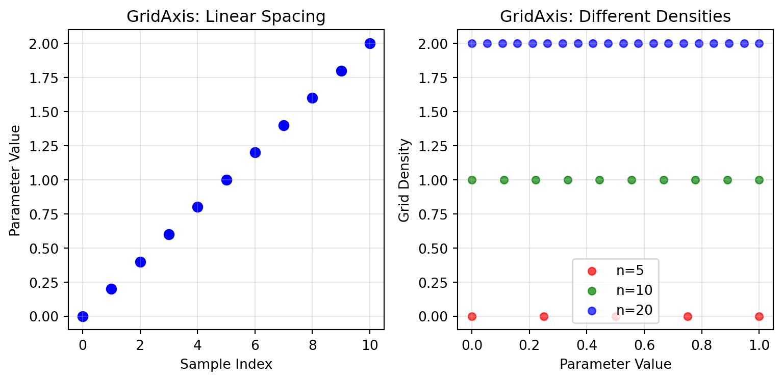
## GridAxis - Deterministic Sampling
GridAxis samples a deterministic grid across a parameter range — identical values every run, no randomness.
```{python}
# Basic grid sampling
grid_basic = GridAxis(0.0, 2.0, 11)
values_basic = grid_basic.generate_values()

print(f"Grid values: {values_basic}")
print(f"Spacing is uniform: {jnp.allclose(jnp.diff(values_basic), jnp.diff(values_basic)[0])}")

# Multiple grid densities
densities = [5, 10, 20]
for n in densities:
    grid = GridAxis(0.0, 1.0, n)
    values = grid.generate_values()
    print(f"n={n:2d}: {len(values)} values from {values[0]:.3f} to {values[-1]:.3f}")
```
```{python}
#| code-fold: true
#| code-summary: "Show visualization code"
# Visualize grid sampling
fig, (ax1, ax2) = plt.subplots(1, 2, figsize=(8.1, 4))

# Plot 1: Basic grid values
ax1.scatter(range(len(values_basic)), values_basic, color='blue', s=50)
ax1.set_xlabel('Sample Index')
ax1.set_ylabel('Parameter Value')
ax1.set_title('GridAxis: Linear Spacing')
ax1.grid(True, alpha=0.3)

# Plot 2: Multiple grid densities
colors = ['red', 'green', 'blue']
for i, (n, color) in enumerate(zip(densities, colors)):
    grid = GridAxis(0.0, 1.0, n)
    values = grid.generate_values()
    ax2.scatter(values, [i] * len(values), color=color, s=30,
               label=f'n={n}', alpha=0.7)

ax2.set_xlabel('Parameter Value')
ax2.set_ylabel('Grid Density')
ax2.set_title('GridAxis: Different Densities')
ax2.legend()
ax2.grid(True, alpha=0.3)

plt.tight_layout()
plt.show()
```
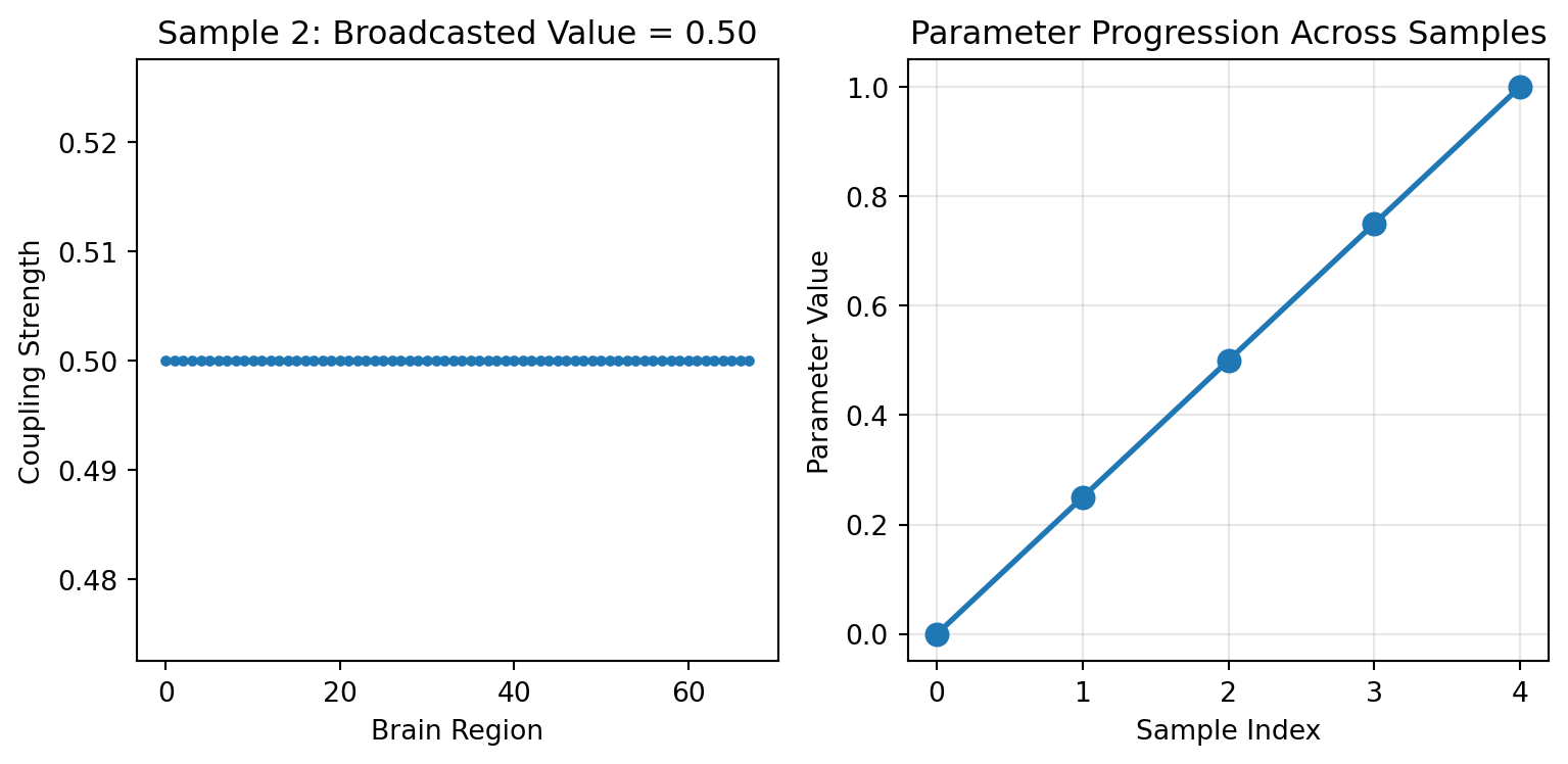
### Shape Broadcasting
GridAxis (and UniformAxis) support a `shape` parameter. Each sample becomes a constant array of that shape — useful for parameters that are shared uniformly across brain regions:
```{python}
# Example: Regional coupling strengths (68 brain regions)
n_regions = 68
regional_grid = GridAxis(0.0, 1.0, 5, shape=(n_regions,))
regional_values = regional_grid.generate_values()

print(f"Regional grid shape: {regional_values.shape}")
print(f"Each sample has shape: {regional_values[0].shape}")
print(f"Sample 2 value: {regional_values[2][0]:.3f} (broadcasted to all regions)")
print(f"All regions identical per sample: {jnp.allclose(regional_values[2], regional_values[2][0])}")
```
```{python}
#| code-fold: true
#| code-summary: "Show visualization code"
# Visualize the broadcasting
fig, (ax1, ax2) = plt.subplots(1, 2, figsize=(8.1, 4))

# Show that each sample broadcasts the same value
sample_idx = 2
ax1.plot(regional_values[sample_idx], 'o-', markersize=3)
ax1.set_xlabel('Brain Region')
ax1.set_ylabel('Coupling Strength')
ax1.set_title(f'Sample {sample_idx}: Broadcasted Value = {regional_values[sample_idx][0]:.2f}')

# Show progression across samples
ax2.plot(range(5), regional_values[:, 0], 'o-', linewidth=2, markersize=8)
ax2.set_xlabel('Sample Index')
ax2.set_ylabel('Parameter Value')
ax2.set_title('Parameter Progression Across Samples')
ax2.grid(True, alpha=0.3)

plt.tight_layout()
plt.show()
```
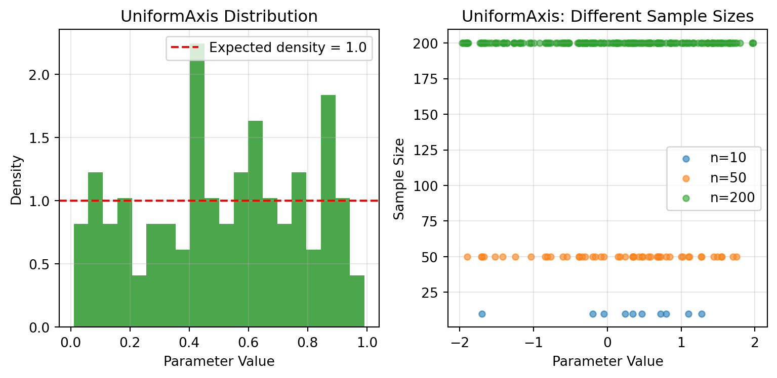
## UniformAxis - Random Sampling
UniformAxis draws samples uniformly at random. Pass the same key and you get identical values.
```{python}
# Reproducible random sampling
key = jax.random.key(42)
uniform = UniformAxis(0.0, 1.0, 100)

values1 = uniform.generate_values(key)
values2 = uniform.generate_values(key)  # Same key = same values
values3 = uniform.generate_values(jax.random.key(43))  # Different key

print(f"Same key gives identical results: {jnp.allclose(values1, values2)}")
print(f"Different key gives different results: {not jnp.allclose(values1, values3)}")
print(f"Mean value: {jnp.mean(values1):.3f} (should be ~0.5)")
print(f"Value range: [{jnp.min(values1):.3f}, {jnp.max(values1):.3f}]")
```
```{python}
#| code-fold: true
#| code-summary: "Show visualization code"
# Visualize distributions
fig, (ax1, ax2) = plt.subplots(1, 2, figsize=(8.1, 4))

# Histogram of uniform samples
ax1.hist(values1, bins=20, alpha=0.7, color='green', density=True)
ax1.axhline(y=1.0, color='red', linestyle='--', label='Expected density = 1.0')
ax1.set_xlabel('Parameter Value')
ax1.set_ylabel('Density')
ax1.set_title('UniformAxis Distribution')
ax1.legend()
ax1.grid(True, alpha=0.3)

# Comparison of different sample sizes
sample_sizes = [10, 50, 200]
for size in sample_sizes:
    uniform_temp = UniformAxis(-2.0, 2.0, size)
    samples = uniform_temp.generate_values(jax.random.key(42))
    ax2.scatter(samples, [size] * len(samples), alpha=0.6, s=20,
               label=f'n={size}')

ax2.set_xlabel('Parameter Value')
ax2.set_ylabel('Sample Size')
ax2.set_title('UniformAxis: Different Sample Sizes')
ax2.legend()
ax2.grid(True, alpha=0.3)

plt.tight_layout()
plt.show()
```
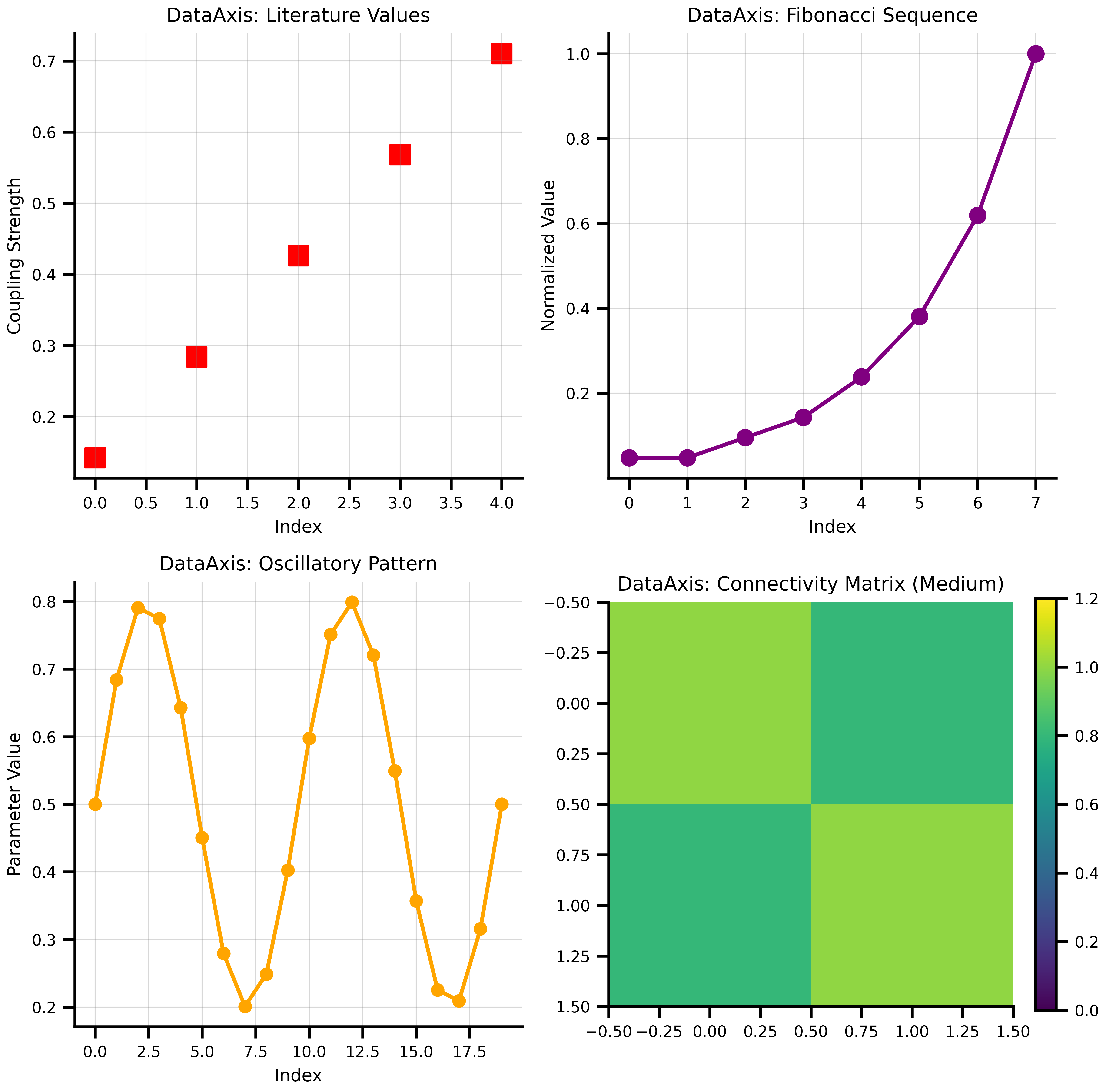
## DataAxis - Predefined Values
DataAxis lets you use predefined sequences of values.
```{python}
# Example: Testing specific coupling values from literature
literature_values = jnp.array([0.142, 0.284, 0.426, 0.568, 0.710])
data_axis = DataAxis(literature_values)

print(f"DataAxis size: {data_axis.size}")
print(f"Values: {data_axis.generate_values()}")

# Works with multidimensional data too
connectivity_matrices = jnp.array([
    [[1.0, 0.5], [0.5, 1.0]],  # Weak coupling
    [[1.0, 0.8], [0.8, 1.0]],  # Medium coupling
    [[1.0, 1.2], [1.2, 1.0]]   # Strong coupling
])

matrix_axis = DataAxis(connectivity_matrices)
print(f"\nMatrix axis shape: {matrix_axis.generate_values().shape}")
print("First connectivity matrix:")
print(matrix_axis.generate_values()[0])

# Create some creative data patterns
fib_values = jnp.array([1, 1, 2, 3, 5, 8, 13, 21])
fib_normalized = fib_values / fib_values.max()
print(f"\nFibonacci sequence (normalized): {fib_normalized}")

# Oscillatory pattern
t = jnp.linspace(0, 4*jnp.pi, 20)
oscillatory = 0.5 + 0.3 * jnp.sin(t)
print(f"Oscillatory pattern range: [{jnp.min(oscillatory):.3f}, {jnp.max(oscillatory):.3f}]")
```
```{python}
#| code-fold: true
#| code-summary: "Show visualization code"
# Visualize different data patterns
fig, axes = plt.subplots(2, 2, figsize=(8.1, 8))

# 1. Literature values
ax = axes[0, 0]
ax.scatter(range(len(literature_values)), literature_values,
          color='red', s=100, marker='s')
ax.set_xlabel('Index')
ax.set_ylabel('Coupling Strength')
ax.set_title('DataAxis: Literature Values')
ax.grid(True, alpha=0.3)

# 2. Fibonacci sequence
fib_axis = DataAxis(fib_normalized)
ax = axes[0, 1]
ax.plot(fib_normalized, 'o-', color='purple', linewidth=2, markersize=8)
ax.set_xlabel('Index')
ax.set_ylabel('Normalized Value')
ax.set_title('DataAxis: Fibonacci Sequence')
ax.grid(True, alpha=0.3)

# 3. Oscillatory pattern
osc_axis = DataAxis(oscillatory)
ax = axes[1, 0]
ax.plot(oscillatory, 'o-', color='orange', linewidth=2, markersize=6)
ax.set_xlabel('Index')
ax.set_ylabel('Parameter Value')
ax.set_title('DataAxis: Oscillatory Pattern')
ax.grid(True, alpha=0.3)

# 4. Connectivity matrix visualization
ax = axes[1, 1]
im = ax.imshow(matrix_axis.generate_values()[1], cmap='viridis', vmin=0, vmax=1.2)
ax.set_title('DataAxis: Connectivity Matrix (Medium)')
plt.colorbar(im, ax=ax, fraction=0.046)

plt.tight_layout()
plt.show()
```
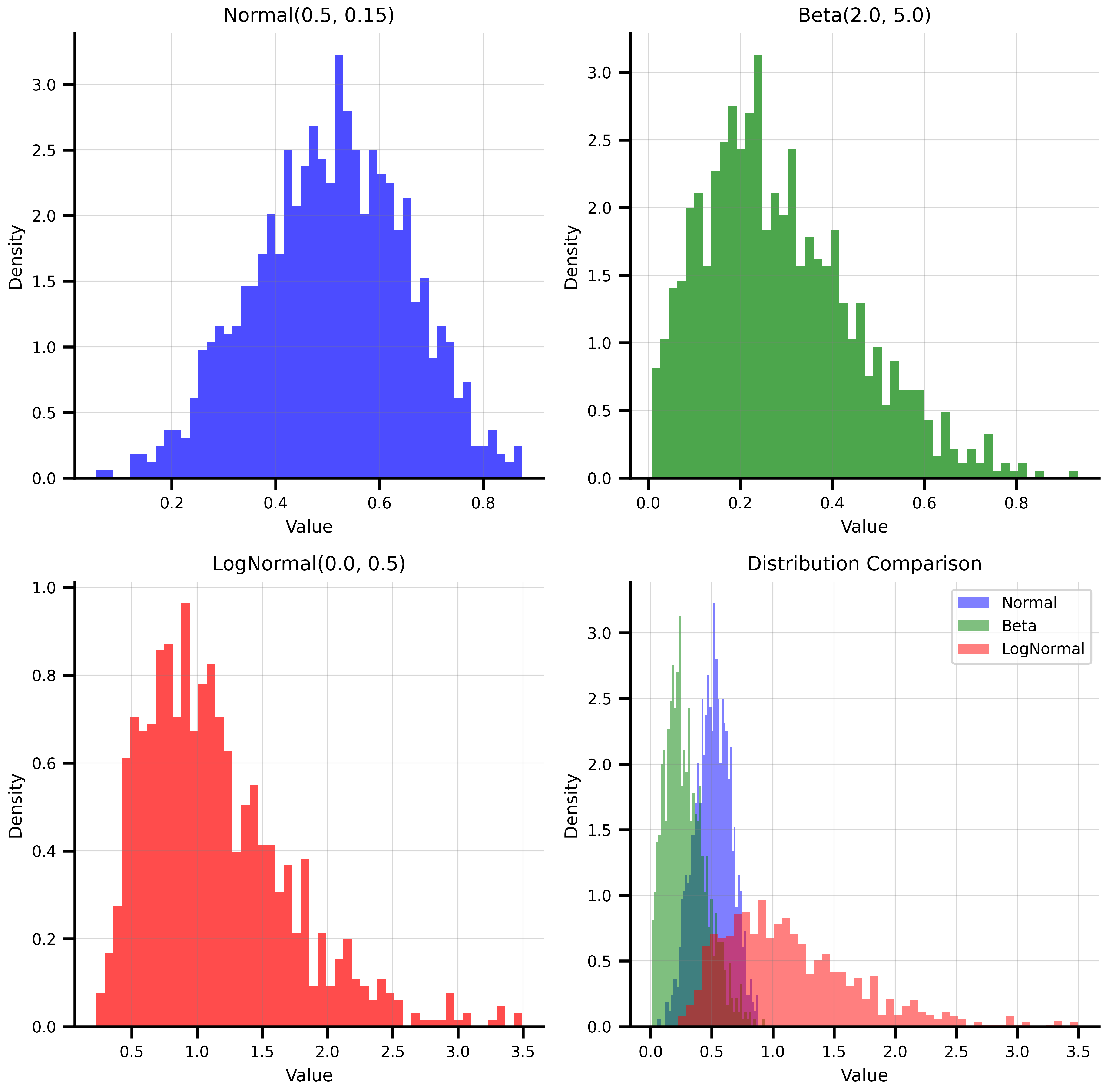
## NumPyroAxis - Distribution Sampling
NumPyroAxis wraps any NumPyro distribution, making it a natural fit for Bayesian workflows and uncertainty quantification.
```{python}
import numpyro.distributions as dist

# Different distribution types
key = jax.random.key(42)

# Normal distribution - common for many biological parameters
normal_axis = NumPyroAxis(dist.Normal(0.5, 0.15), n=1000)
normal_samples = normal_axis.generate_values(key)

# Beta distribution - great for bounded parameters [0,1]
beta_axis = NumPyroAxis(dist.Beta(2.0, 5.0), n=1000)
beta_samples = beta_axis.generate_values(key)

# LogNormal - for positive-only parameters like time constants
lognormal_axis = NumPyroAxis(dist.LogNormal(0.0, 0.5), n=1000)
lognormal_samples = lognormal_axis.generate_values(key)

print(f"Normal samples: mean={jnp.mean(normal_samples):.3f}, std={jnp.std(normal_samples):.3f}")
print(f"Beta samples: mean={jnp.mean(beta_samples):.3f}, range=[{jnp.min(beta_samples):.3f}, {jnp.max(beta_samples):.3f}]")
print(f"LogNormal samples: mean={jnp.mean(lognormal_samples):.3f}, median={jnp.median(lognormal_samples):.3f}")
```
```{python}
#| code-fold: true
#| code-summary: "Show visualization code"
# Visualize the distributions
fig, axes = plt.subplots(2, 2, figsize=(8.1, 8))

# Normal distribution
ax = axes[0, 0]
ax.hist(normal_samples, bins=50, density=True, alpha=0.7, color='blue')
ax.set_xlabel('Value')
ax.set_ylabel('Density')
ax.set_title('Normal(0.5, 0.15)')
ax.grid(True, alpha=0.3)

# Beta distribution
ax = axes[0, 1]
ax.hist(beta_samples, bins=50, density=True, alpha=0.7, color='green')
ax.set_xlabel('Value')
ax.set_ylabel('Density')
ax.set_title('Beta(2.0, 5.0)')
ax.grid(True, alpha=0.3)

# LogNormal distribution
ax = axes[1, 0]
ax.hist(lognormal_samples, bins=50, density=True, alpha=0.7, color='red')
ax.set_xlabel('Value')
ax.set_ylabel('Density')
ax.set_title('LogNormal(0.0, 0.5)')
ax.grid(True, alpha=0.3)

# Comparison of all three
ax = axes[1, 1]
ax.hist(normal_samples, bins=50, density=True, alpha=0.5, color='blue', label='Normal')
ax.hist(beta_samples, bins=50, density=True, alpha=0.5, color='green', label='Beta')
ax.hist(lognormal_samples[lognormal_samples < 5], bins=50, density=True, alpha=0.5, color='red', label='LogNormal')
ax.set_xlabel('Value')
ax.set_ylabel('Density')
ax.set_title('Distribution Comparison')
ax.legend()
ax.grid(True, alpha=0.3)

plt.tight_layout()
plt.show()
```
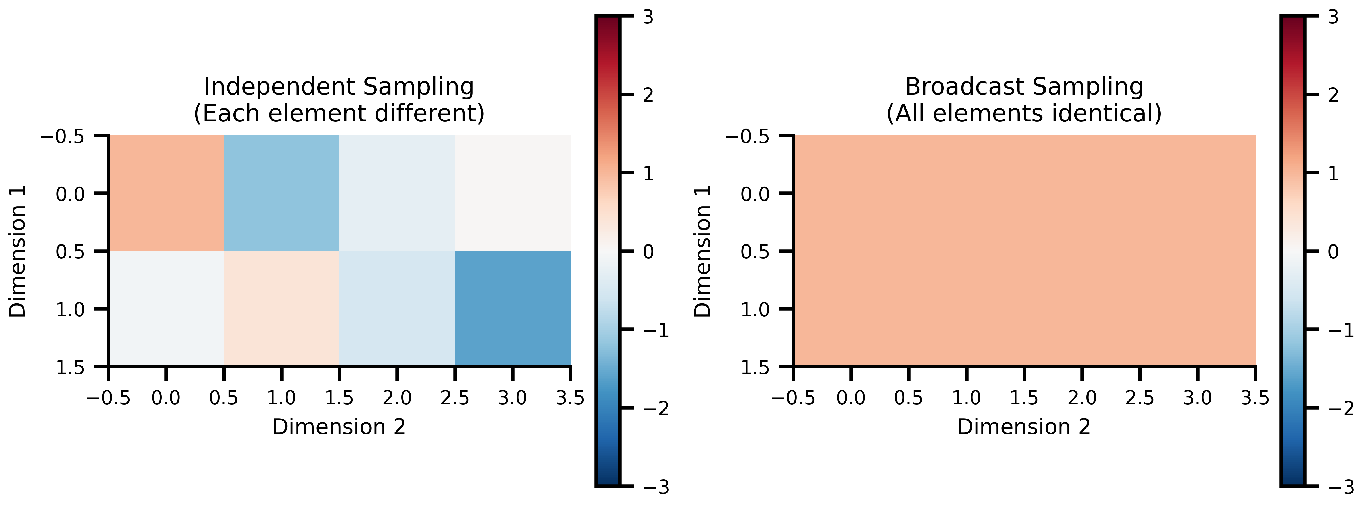
### Independent vs Broadcast Sampling
NumPyroAxis supports two sampling modes for different modeling scenarios:
```{python}
key = jax.random.key(456)

# Independent mode: each element sampled independently
independent_axis = NumPyroAxis(
    dist.Normal(0.0, 1.0),
    n=3,
    sample_shape=(2, 4),
    broadcast_mode=False
)
independent_samples = independent_axis.generate_values(key)

# Broadcast mode: one sample per axis point, broadcast to shape
broadcast_axis = NumPyroAxis(
    dist.Normal(0.0, 1.0),
    n=3,
    sample_shape=(2, 4),
    broadcast_mode=True
)
broadcast_samples = broadcast_axis.generate_values(key)

print("Independent sampling:")
print(f"Shape: {independent_samples.shape}")
print("Sample 0 (each element different):")
print(independent_samples[0])
print()

print("Broadcast sampling:")
print(f"Shape: {broadcast_samples.shape}")
print("Sample 0 (all elements identical):")
print(broadcast_samples[0])
print(f"All elements identical: {jnp.allclose(broadcast_samples[0], broadcast_samples[0].flatten()[0])}")
```
```{python}
#| code-fold: true
#| code-summary: "Show visualization code"
# Visualize the difference
fig, (ax1, ax2) = plt.subplots(1, 2, figsize=(8.1, 4))

# Independent sampling heatmap
im1 = ax1.imshow(independent_samples[0], cmap='RdBu_r', vmin=-3, vmax=3)
ax1.set_title('Independent Sampling\n(Each element different)')
ax1.set_xlabel('Dimension 2')
ax1.set_ylabel('Dimension 1')
plt.colorbar(im1, ax=ax1, fraction=0.046)

# Broadcast sampling heatmap
im2 = ax2.imshow(broadcast_samples[0], cmap='RdBu_r', vmin=-3, vmax=3)
ax2.set_title('Broadcast Sampling\n(All elements identical)')
ax2.set_xlabel('Dimension 2')
ax2.set_ylabel('Dimension 1')
plt.colorbar(im2, ax=ax2, fraction=0.046)

plt.tight_layout()
plt.show()
```
# Composing with Space
## Basic Space Creation
Space takes a state tree — axes where you want variation, plain values where you don't — and generates all parameter combinations from it.
```{python}
# Create a realistic brain simulation parameter space
simulation_state = {
    'coupling': {
        'strength': GridAxis(0.1, 0.8, 5),      # Coupling strength
        'delay': UniformAxis(5.0, 25.0, 3),     # Transmission delays (ms)
    },
    'model': {
        'noise_amplitude': DataAxis([0.01, 0.02, 0.05]),  # Noise levels from pilot study
        'time_constant': 10.0,                    # Fixed parameter
    },
    'simulation': {
        'dt': 0.1,                               # Fixed time step
        'duration': 1000,                        # Fixed duration
    }
}

# Create the space
space = Space(simulation_state, mode='product', key=jax.random.key(789))
print(f"Parameter space contains {len(space)} combinations")
print(f"Combination modes: 5 × 3 × 3 = {5*3*3} (Grid × Uniform × Data)")

# Look at a few parameter combinations
print("\nFirst 3 parameter combinations:")
print("=" * 50)

for i, params in enumerate(space):
    if i >= 3: break
    print(f"\nCombination {i}:")
    print(f"  Coupling strength: {params['coupling']['strength']:.3f}")
    print(f"  Coupling delay: {params['coupling']['delay']:.2f} ms")
    print(f"  Noise amplitude: {params['model']['noise_amplitude']:.3f}")
    print(f"  Time constant: {params['model']['time_constant']} (fixed)")
    print(f"  Simulation dt: {params['simulation']['dt']} (fixed)")
```
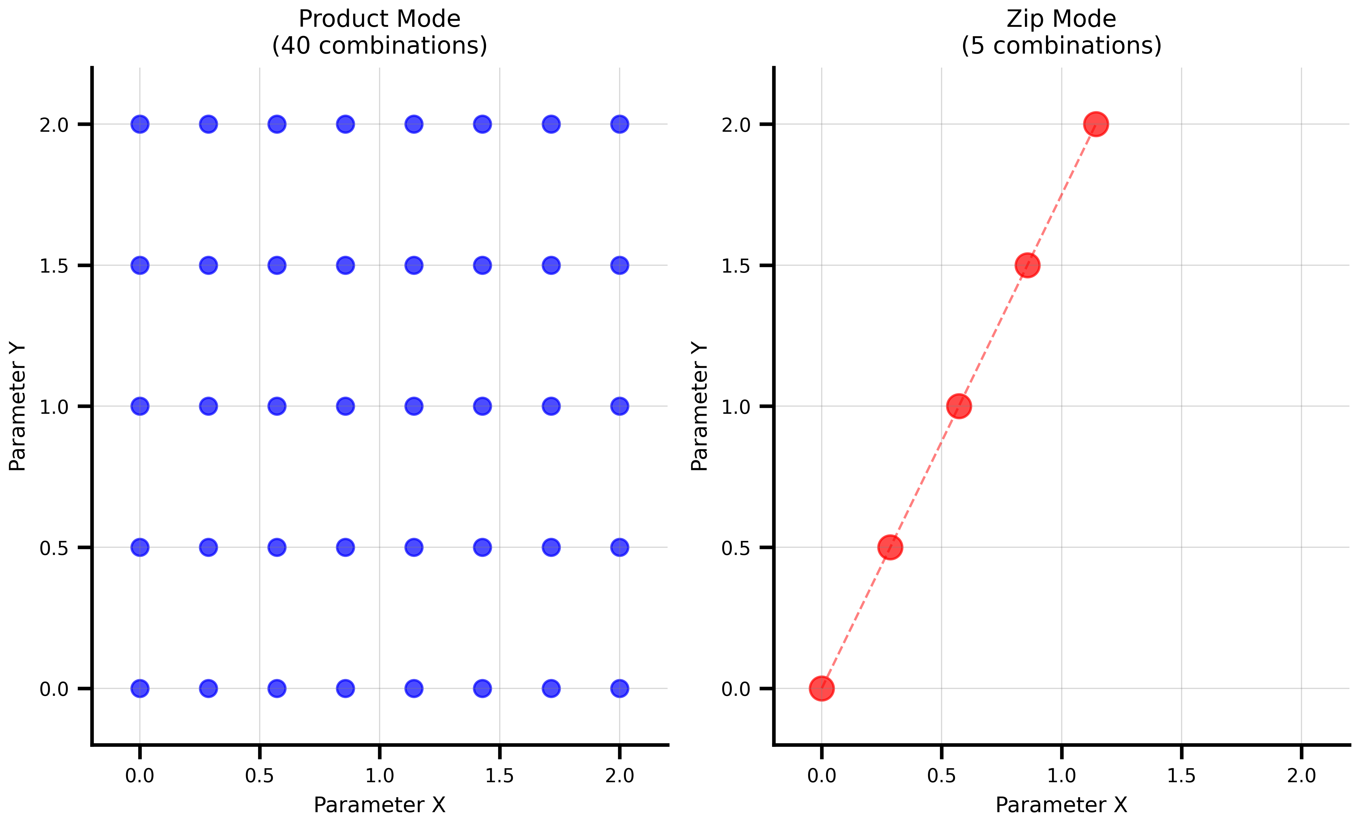
## Combination Modes: Product vs Zip
The two combination modes serve different exploration strategies:
### Product Mode (Cartesian Product)
Tests every combination of parameter values. Use this for systematic exploration.
```{python}
# Product mode: systematic exploration
product_state = {
    'param_a': GridAxis(0.0, 1.0, 3),
    'param_b': GridAxis(0.0, 1.0, 2),
}

product_space = Space(product_state, mode='product')
print(f"Product mode: {len(product_space)} combinations")

print("\nAll combinations (product mode):")
for i, params in enumerate(product_space):
    print(f"  {i}: a={params['param_a']:.1f}, b={params['param_b']:.1f}")
```
### Zip Mode (Parallel Sampling)
Pairs corresponding elements from each axis. Use this when parameters must move together.
```{python}
# Zip mode: matched sampling
zip_space = Space(product_state, mode='zip')
print(f"Zip mode: {len(zip_space)} combinations (uses minimum axis size)")

print("\nMatched combinations (zip mode):")
for i, params in enumerate(zip_space):
    print(f"  {i}: a={params['param_a']:.1f}, b={params['param_b']:.1f}")
```
```{python}
#| code-fold: true
#| code-summary: "Show visualization code"
# Create a more interesting comparison
comparison_state = {
    'x': GridAxis(0.0, 2.0, 8),
    'y': GridAxis(0.0, 2.0, 5),
}

product_comp = Space(comparison_state, mode='product')
zip_comp = Space(comparison_state, mode='zip')

# Extract coordinates for plotting
product_x = [p['x'] for p in product_comp]
product_y = [p['y'] for p in product_comp]

zip_x = [p['x'] for p in zip_comp]
zip_y = [p['y'] for p in zip_comp]

fig, (ax1, ax2) = plt.subplots(1, 2, figsize=(8.1, 5))

# Product mode visualization
ax1.scatter(product_x, product_y, color='blue', s=50, alpha=0.7)
ax1.set_xlabel('Parameter X')
ax1.set_ylabel('Parameter Y')
ax1.set_title(f'Product Mode\n({len(product_comp)} combinations)')
ax1.grid(True, alpha=0.3)
ax1.set_xlim(-0.2, 2.2)
ax1.set_ylim(-0.2, 2.2)

# Zip mode visualization
ax2.scatter(zip_x, zip_y, color='red', s=100, alpha=0.7)
ax2.plot(zip_x, zip_y, 'r--', alpha=0.5, linewidth=1)
ax2.set_xlabel('Parameter X')
ax2.set_ylabel('Parameter Y')
ax2.set_title(f'Zip Mode\n({len(zip_comp)} combinations)')
ax2.grid(True, alpha=0.3)
ax2.set_xlim(-0.2, 2.2)
ax2.set_ylim(-0.2, 2.2)

plt.tight_layout()
plt.show()
```
## Grouped Axes: Mixing Combination Modes
In many real-world scenarios, you need **both** zip and product behavior in the same space. For example, you might have matched experimental settings that must move in lockstep, combined with a parameter grid you want to explore exhaustively.
The `group` parameter on axes solves this. Axes sharing the same `group` label are **zipped together** into a single composite axis, regardless of where they sit in the state tree. Then all groups and ungrouped axes combine using the Space's mode (typically product).
### Basic Example
```{python}
# Three matched settings that must stay together
setting_values_a = jnp.array([1.0, 2.0, 3.0])
setting_values_b = jnp.array([10.0, 20.0, 30.0])

grouped_state = {
    'setting_a': DataAxis(setting_values_a, group='settings'),
    'setting_b': DataAxis(setting_values_b, group='settings'),
    'param_x': GridAxis(0.0, 1.0, 4),
}

space = Space(grouped_state, mode='product', key=jax.random.key(42))
print(f"Total combinations: {len(space)}")
print(f"  = 3 settings x 4 param_x = {3 * 4}")
print(f"  (NOT 3 x 3 x 4 = {3 * 3 * 4})")

print("\nAll combinations:")
for i, params in enumerate(space):
    print(f"  {i}: setting_a={params['setting_a']:.0f}, "
          f"setting_b={params['setting_b']:.0f}, "
          f"param_x={params['param_x']:.2f}")
```
Notice that `setting_a` and `setting_b` always move together (1 with 10, 2 with 20, 3 with 30) while `param_x` varies independently across its full grid.
Groups work across subtrees -- grouped axes don't need to be co-located in the state tree. You can also use multiple independent groups (each with its own label), and they each zip internally before being combined via the Space's mode. The `group` label can be any hashable value (strings, ints, tuples, etc.).
## Iteration & Access Patterns
Space supports standard Python iteration, integer indexing (including negative), and slicing. Slices return a new Space.
```{python}
demo_state = {
    'coupling': GridAxis(0.0, 1.0, 6),
    'noise': UniformAxis(0.01, 0.1, 6),
    'threshold': 0.5
}
demo_space = Space(demo_state, mode='zip', key=jax.random.key(42))

# Iterate
for i, params in enumerate(demo_space):
    if i >= 3: break
    print(f"  {i}: coupling={params['coupling']:.2f}, noise={params['noise']:.4f}")

# Index and slice
print(demo_space[0]['coupling'], demo_space[-1]['coupling'])
subset = demo_space[1:4]
print(f"Subset: {len(subset)} combinations")
```
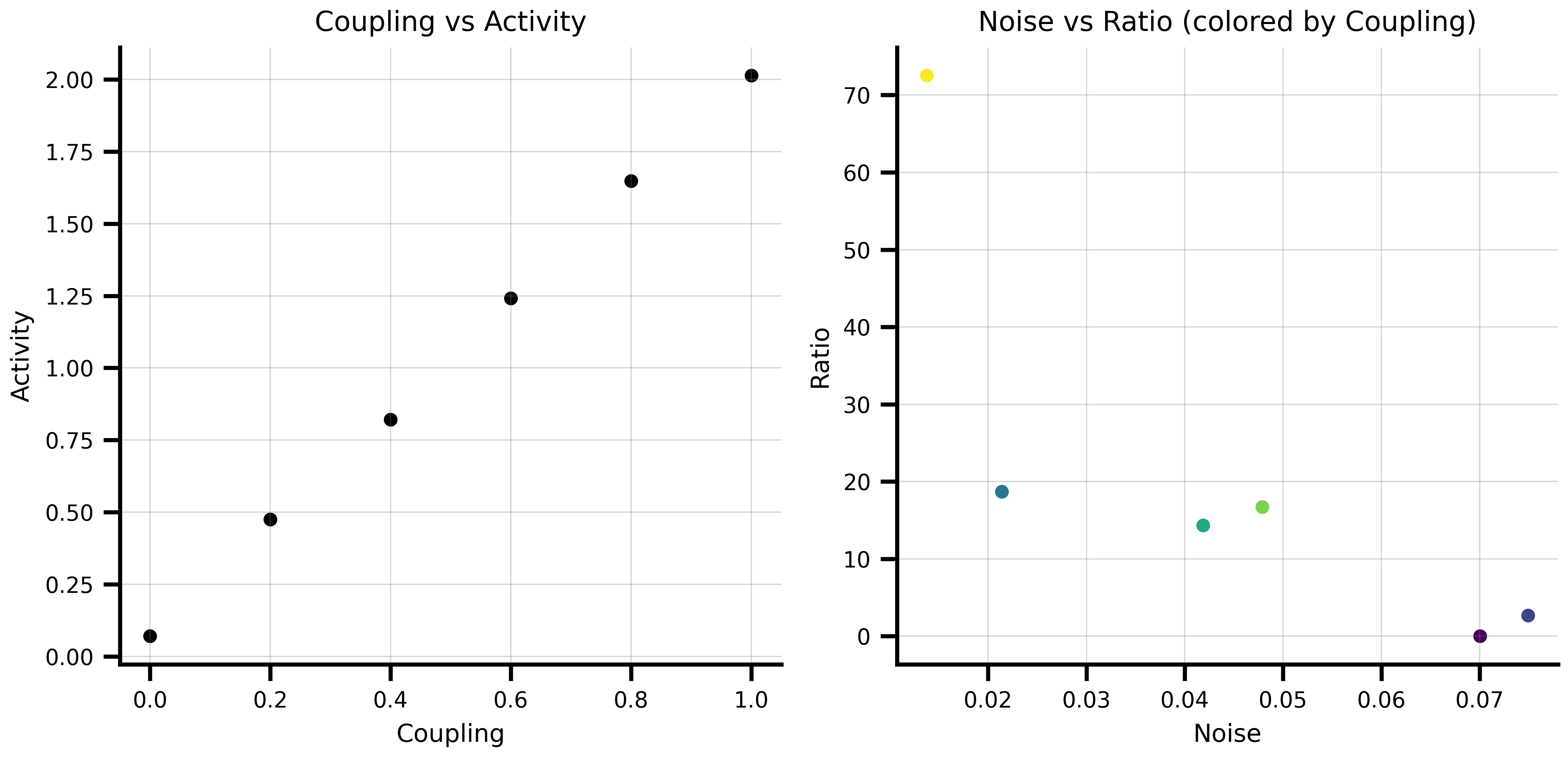
### Converting to DataFrames
Both spaces and execution results can be converted to pandas DataFrames for easy analysis and plotting. Column names are derived automatically from the pytree structure of your state.
```{python}
# Parameter space as a DataFrame
df_params = demo_space.to_dataframe()
print(df_params.head())
```
After running a computation, `Result.to_dataframe()` combines parameters and results into a single DataFrame, keeping them correctly aligned:
```{python}
from tvboptim.execution import SequentialExecution

def compute_metric(state):
    return {'activity': state['coupling'] * 2 + state['noise'],
            'ratio': state['coupling'] / (state['noise'] + 1e-6)}

result = SequentialExecution(compute_metric, demo_space).run()
df = result.to_dataframe()
print(df.head())
```
```{python}
#| code-fold: true
#| code-summary: "Show plotting example"
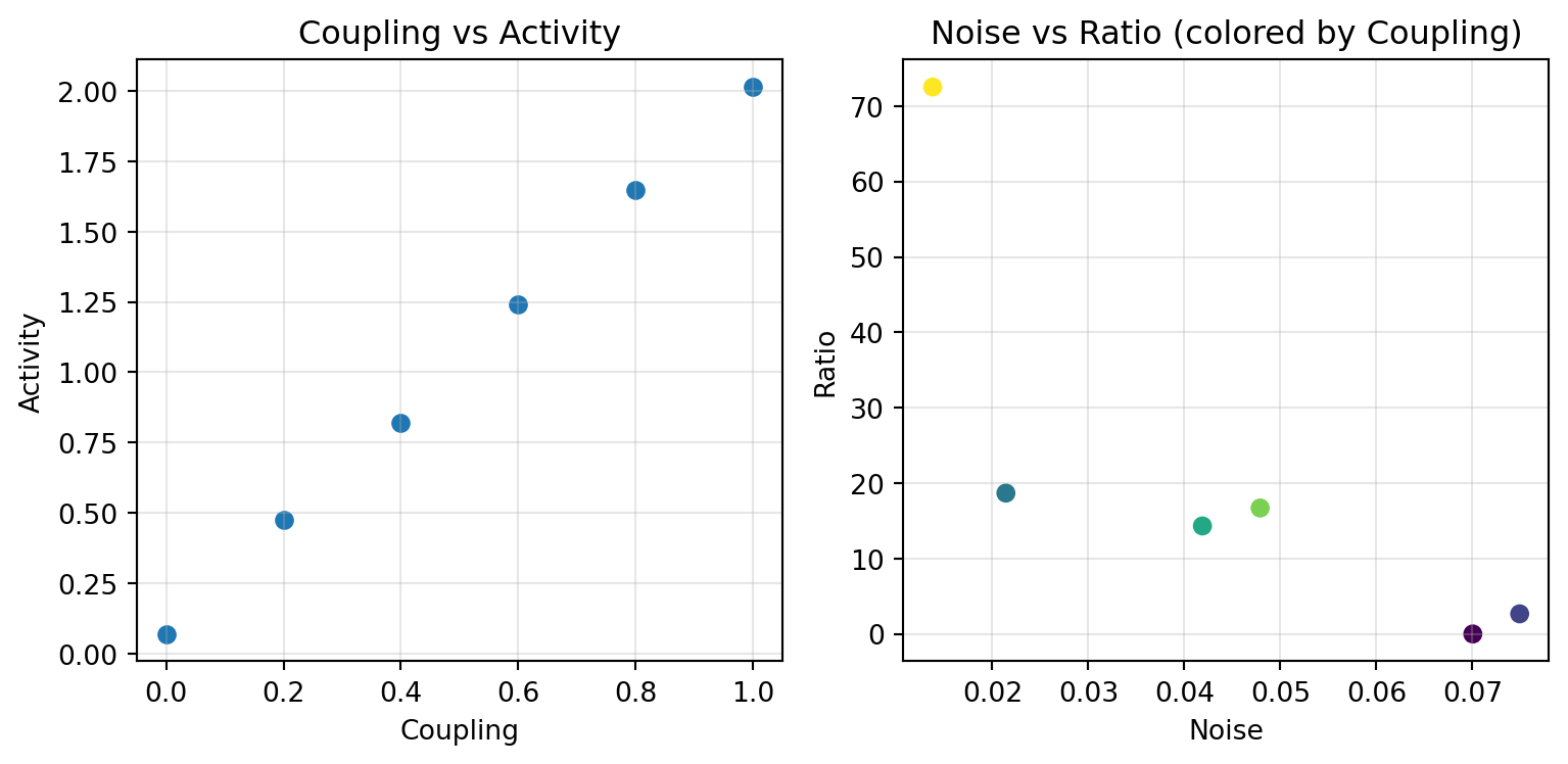
fig, (ax1, ax2) = plt.subplots(1, 2, figsize=(8.1, 4))

ax1.scatter(df['coupling'], df['activity'])
ax1.set_xlabel('Coupling')
ax1.set_ylabel('Activity')
ax1.set_title('Coupling vs Activity')
ax1.grid(True, alpha=0.3)

ax2.scatter(df['noise'], df['ratio'], c=df['coupling'], cmap='viridis')
ax2.set_xlabel('Noise')
ax2.set_ylabel('Ratio')
ax2.set_title('Noise vs Ratio (colored by Coupling)')
ax2.grid(True, alpha=0.3)

plt.tight_layout()
plt.show()
```
Nested state structures produce dot-separated column names (e.g. `model.G`, `noise.sigma`), and non-scalar results like arrays or matrices are stored as object cells in the DataFrame.
# Execution: Running Functions Over Spaces
The axis and space system works with any pure JAX function — not just TVB network models. The examples here use a real brain network, which is the typical use case.
```{python}
import copy
from tvboptim.execution import SequentialExecution, ParallelExecution
from tvboptim.experimental.network_dynamics import Network, prepare
from tvboptim.experimental.network_dynamics.dynamics.tvb import ReducedWongWang
from tvboptim.experimental.network_dynamics.coupling import LinearCoupling
from tvboptim.experimental.network_dynamics.graph import DenseGraph
from tvboptim.experimental.network_dynamics.noise import AdditiveNoise
from tvboptim.experimental.network_dynamics.solvers import Heun

n_nodes = 8
network = Network(
    dynamics=ReducedWongWang(),
    coupling={'instant': LinearCoupling(incoming_states='S', G=0.5)},
    graph=DenseGraph(jnp.ones((n_nodes, n_nodes)) - jnp.eye(n_nodes)),
    noise=AdditiveNoise(sigma=1e-3, key=jax.random.key(0)),
)
solve_fn, base_cfg = prepare(network, Heun(), t0=0.0, t1=5.0, dt=0.1)
print(f"Prepared: {n_nodes}-node RWW network, {int(5.0/0.1)} time steps")
```
`prepare` returns a compiled solve function and a config object. Axes attach directly to config leaves — `solve_fn` stays constant across the whole sweep.
```{python}
def observe(cfg):
    ys = solve_fn(cfg).ys  # shape: [n_steps, n_state_vars, n_nodes]
    return {'mean_S': ys.mean(), 'std_S': ys.std()}
```
## Sequential Execution
Sequential execution processes one parameter combination at a time. Use it for debugging, memory-constrained environments, or when your model doesn't vectorize cleanly.
```{python}
seq_state = copy.deepcopy(base_cfg)
seq_state.coupling.instant.G = GridAxis(0.1, 1.0, 8)

seq_space = Space(seq_state, mode='product')
seq_results = SequentialExecution(observe, seq_space).run()

df_seq = seq_results.to_dataframe()
print(df_seq)
```
```{python}
#| code-fold: true
#| code-summary: "Show visualization code"
fig, (ax1, ax2) = plt.subplots(1, 2, figsize=(8.1, 4))

ax1.plot(df_seq['coupling.instant.G'], df_seq['mean_S'], 'o-')
ax1.set_xlabel('Coupling G')
ax1.set_ylabel('Mean S')
ax1.set_title('Mean activity vs coupling strength')
ax1.grid(True, alpha=0.3)

ax2.plot(df_seq['coupling.instant.G'], df_seq['std_S'], 'o-', color='orange')
ax2.set_xlabel('Coupling G')
ax2.set_ylabel('Std S')
ax2.set_title('Activity variability vs coupling strength')
ax2.grid(True, alpha=0.3)

plt.tight_layout()
plt.show()
```
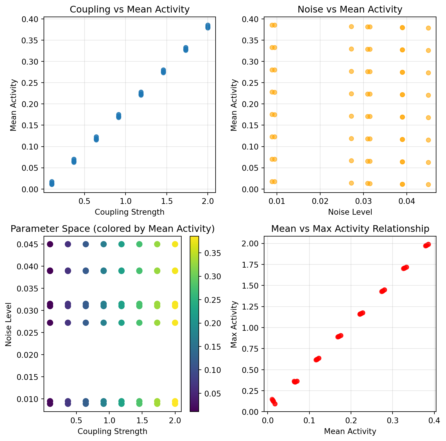
## Parallel Execution
Parallel execution uses JAX's `pmap` and `vmap` for vectorized computation across multiple devices. With large parameter spaces, this is where the runtime difference becomes significant.
```{python}
par_state = copy.deepcopy(base_cfg)
par_state.coupling.instant.G = GridAxis(0.1, 1.0, 8)
par_state.noise.sigma = GridAxis(1e-4, 5e-3, 4)

par_space = Space(par_state, mode='product')  # 8 × 4 = 32 combinations
print(f"Parameter space: {len(par_space)} combinations")

par_results = ParallelExecution(observe, par_space, n_vmap=8, n_pmap=1).run()
print(f"Done: {len(par_results)} results")
```
```{python}
#| code-fold: true
#| code-summary: "Show visualization code"
df_par = par_results.to_dataframe()

fig, (ax1, ax2) = plt.subplots(1, 2, figsize=(8.1, 4))

for sigma, group in df_par.groupby('noise.sigma'):
    ax1.plot(group['coupling.instant.G'], group['mean_S'],
             'o-', alpha=0.7, label=f'σ={sigma:.4f}')
ax1.set_xlabel('Coupling G')
ax1.set_ylabel('Mean S')
ax1.set_title('G sweep across noise amplitudes')
ax1.legend(fontsize=8)
ax1.grid(True, alpha=0.3)

scatter = ax2.scatter(df_par['coupling.instant.G'], df_par['mean_S'],
                      c=df_par['noise.sigma'], cmap='plasma', s=40)
ax2.set_xlabel('Coupling G')
ax2.set_ylabel('Mean S')
ax2.set_title('Mean S across parameter space')
plt.colorbar(scatter, ax=ax2, label='noise σ')
ax2.grid(True, alpha=0.3)

plt.tight_layout()
plt.show()
```
## Performance Comparison
For trivial models the JIT and dispatch overhead of parallel execution outweighs the speedup — sequential wins at small scale. The crossover depends on model complexity and problem size.
```{python}
import time

timing_state = {
    'param1': GridAxis(0.0, 1.0, 5),
    'param2': UniformAxis(0.0, 1.0, 5)
}
timing_space = Space(timing_state, mode='product', key=jax.random.key(789))

def simple_model(state):
    return {'result': state['param1'] * state['param2']}

print("Performance comparison on 25 parameter combinations:")
print("=" * 55)

seq_exec = SequentialExecution(simple_model, timing_space)
start = time.time()
seq_results = seq_exec.run()
seq_time = time.time() - start
print(f"Sequential execution: {seq_time:.4f} seconds")

par_exec = ParallelExecution(simple_model, timing_space, n_vmap=5, n_pmap=1)
start = time.time()
par_results = par_exec.run()
par_time = time.time() - start
print(f"Parallel execution:   {par_time:.4f} seconds")

if seq_time > par_time:
    print(f"Parallel speedup:     {seq_time / par_time:.1f}x faster")
else:
    print("Sequential was faster (overhead dominates for small problems)")
```
### When to Use Each Approach
**Sequential Execution:**
- **Debugging**: Easy to trace through individual parameter combinations
- **Memory constraints**: Processes one combination at a time
- **Complex models**: When models don't easily vectorize
- **Small parameter spaces**: Overhead of parallelization not worth it
**Parallel Execution:**
- **Large parameter spaces**: Massive speedups for hundreds/thousands of combinations
- **JAX-compatible models**: Models that can be easily vectorized
- **Production runs**: When you need results fast
- **Multi-device setups**: Can use multiple GPUs/TPUs
### Integration with Spaces
Both execution types work with all space features. Any axis type can be placed on any config leaf:
```{python}
mixed_state = copy.deepcopy(base_cfg)
mixed_state.coupling.instant.G = NumPyroAxis(dist.Beta(2.0, 5.0), n=4)
mixed_state.noise.sigma = DataAxis(jnp.array([1e-4, 5e-4, 1e-3]))

mixed_space = Space(mixed_state, mode='product', key=jax.random.key(0))
print(f"{len(mixed_space)} combinations (4 coupling samples × 3 noise levels)")

result = SequentialExecution(observe, mixed_space).run()
print(result.to_dataframe())
```
# Scanning Noise Seeds for Stochastic Simulations
When the model is stochastic (a `Network` with an `AbstractNoise` attached, integrated with a native solver), the PRNG key that drives the per-step noise increments lives at `config.noise.key`. Because the key is a regular leaf on the prepared config, you can place an axis on it the same way you place axes on any other parameter — no wrapper function, no per-point key swapping. The axis system substitutes the leaf with the per-point value before each call.
```{python}
# Attach axes directly to the config — the leaves they target are
# substituted with per-point values at execution time.
grid_state = copy.deepcopy(base_cfg)
grid_state.coupling.instant.G = GridAxis(0.3, 1.5, 8)                       # Coupling sweep
grid_state.noise.key          = DataAxis(jax.random.split(jax.random.key(0), 8))  # Noise replicates

space = Space(grid_state, mode='product')

def observation(cfg):
    return solve_fn(cfg).ys.mean()

observations = ParallelExecution(observation, space, n_vmap=8, n_pmap=1).run()
```
Two things to know:
- **No re-`prepare` per seed.** The PRNG key is a config leaf, so the axis system substitutes it like any other parameter. `jax.vmap` over the resulting key batch dimension batches the single `jax.random.normal(config.noise.key, ...)` call inside the solve function, with no compile churn beyond the initial JIT.
- **Common random numbers across parameter sweeps.** Place the `DataAxis` of keys on its own (so it shares one key across all `G` values), or use `mode='zip'` to pair them — every `G` point then sees the same realised noise trajectory. This is the classic variance-reduction trick for finite-difference sensitivity estimates.
For workflows that need the increments materialised as an addressable tensor (NumPyro inference over Brownian increments, deterministic replay of a recorded trajectory), populate `config._internal.noise_samples` with an array of shape `[n_steps, n_noise_states, n_nodes]`. The scan branches on this field at trace time and uses it in place of in-scan sampling. Flipping between `None` and an array triggers a one-time JIT retrace. The injection slot is native-only — the Diffrax dispatch supports the same `config.noise.key` swap pattern shown above, but its `VirtualBrownianTree` cannot consume a pre-sampled array.