---
title: "Dynamics"
format:
html:
code-fold: false
toc: true
toc-depth: 3
fig-width: 8
out-width: "100%"
bibliography: references.bib
jupyter: python3
execute:
cache: true
---
# Introduction
Dynamics define the local differential equations governing state evolution at each network node. In brain network modeling, these typically represent neural mass models, population dynamics, or abstract oscillators that capture key features of neural activity.
Each dynamics model specifies:
- **State variables**: Quantities integrated over time (e.g., membrane potential, synaptic gating)
- **Parameters**: Biophysical constants and model-specific coefficients
- **Auxiliary variables**: Derived quantities computed but not integrated (e.g., firing rates)
- **Coupling inputs**: How the model receives input from other nodes
- **External inputs**: How the model receives input from the environment
The general form is:
$$
\frac{d\mathbf{X}}{dt} = f(\mathbf{X}, \text{params}, \text{coupling}, \text{external})
$$
where $\mathbf{X}$ represents state variables at a given node.
# Using Built-in Dynamics
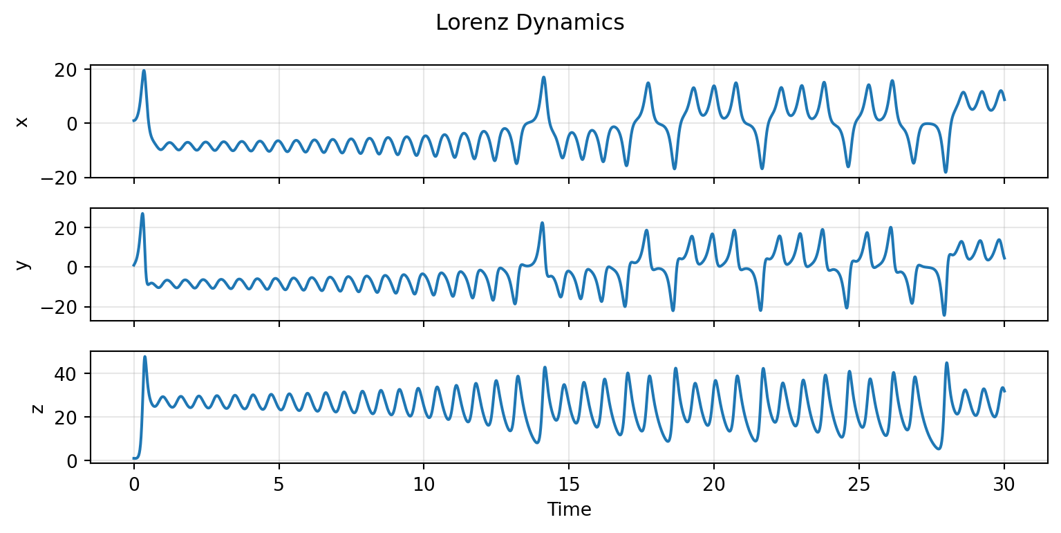
TVB-Optim provides several canonical dynamics models. Let's start with the Lorenz system - a well-known chaotic attractor useful for testing and demonstrating core concepts.
## Standalone Simulation: Lorenz System
```{python}
import jax.numpy as jnp
from tvboptim.experimental.network_dynamics.dynamics import Lorenz

# Create dynamics with default parameters
dynamics = Lorenz()

print(f"State variables: {dynamics.STATE_NAMES}")
print(f"Initial state: {dynamics.INITIAL_STATE}")
print(f"Parameters: {dynamics.params}")
```
The `AbstractDynamics` base class provides methods for standalone testing and visualization:
```{python}
# Verify implementation is correct
dynamics.verify(n_nodes=1)
```
```{python}
# Use built-in plot method
dynamics.plot(t0=0.0, t1=30.0, dt=0.01, n_nodes=1, figsize=(8.1, 4.05))
```
The Lorenz system exhibits deterministic chaos - the characteristic butterfly attractor emerges from sensitivity to initial conditions despite fully deterministic equations.
# The AbstractDynamics Interface
All dynamics models inherit from `AbstractDynamics` and define these class attributes:
```python
from tvboptim.experimental.network_dynamics.core.bunch import Bunch
from tvboptim.experimental.network_dynamics.dynamics.base import AbstractDynamics

class MyDynamics(AbstractDynamics):
    # Required: state variable names and initial values
    STATE_NAMES = ("V", "W")
    INITIAL_STATE = (-0.7, 0.0)

    # Optional: auxiliary variables (computed but not integrated)
    AUXILIARY_NAMES = ("I_mem",)

    # Parameters with defaults
    DEFAULT_PARAMS = Bunch(
        a=0.7,
        b=0.8,
        tau=12.5
    )

    # Declare expected coupling inputs
    COUPLING_INPUTS = {
        'instant': 1,   # 1-dimensional instantaneous coupling
        'delayed': 1    # 1-dimensional delayed coupling
    }

    # Optional: external inputs
    EXTERNAL_INPUTS = {
        'stimulus': 1   # 1-dimensional external stimulus
    }

    # Optional: which variables to record (empty = state variables only)
    VARIABLES_OF_INTEREST = ()
```
## Key Attributes
**State Variables** (`STATE_NAMES`, `INITIAL_STATE`): Quantities integrated over time. These define the dimensionality of the dynamical system.
**Auxiliary Variables** (`AUXILIARY_NAMES`): Derived quantities computed from states but not integrated (e.g., firing rates, membrane currents). Useful for analysis and visualization.
**Parameters** (`DEFAULT_PARAMS`): Model-specific constants that can be overridden at instantiation.
**Coupling Inputs** (`COUPLING_INPUTS`): Declares which named coupling inputs the model expects and their dimensionality. Missing couplings are automatically filled with zeros.
**Variables of Interest** (`VARIABLES_OF_INTEREST`): Controls which variables are saved during simulation:
- **Empty (default)**: Only state variables are recorded
- **Explicit list**: Save specific variables by name or index, including auxiliaries
This is important because auxiliary variables are computed at each time step but **only saved if explicitly included** in `VARIABLES_OF_INTEREST`.
## The dynamics() Method
The core method to implement computes state derivatives (and optionally auxiliary variables):
```python
def dynamics(
    self,
    t: float,                    # Current time
    state: jnp.ndarray,          # [n_states, n_nodes]
    params: Bunch,               # Model parameters
    coupling: Bunch,             # Named coupling inputs
    external: Bunch              # Named external inputs
) -> Union[jnp.ndarray, Tuple[jnp.ndarray, jnp.ndarray]]:
    """
    Returns:
        If no auxiliaries: derivatives [n_states, n_nodes]
        If auxiliaries: (derivatives, auxiliaries) tuple
    """
    # Extract states
    V, W = state[0], state[1]

    # Access coupling by name (filled with zeros if not provided)
    c_instant = coupling.instant[0]

    # Compute auxiliary variables
    I_mem = V - W  # Example membrane current

    # Compute derivatives
    dV_dt = ...
    dW_dt = ...

    # Return derivatives and auxiliaries
    derivatives = jnp.array([dV_dt, dW_dt])
    auxiliaries = jnp.array([I_mem])

    return derivatives, auxiliaries
```
# Creating Custom Dynamics
Let's implement the FitzHugh-Nagumo model [@FitzHugh1961; @Nagumo1962] - a classic 2D reduction of the Hodgkin-Huxley equations that captures excitable neuron dynamics.
The model describes membrane potential $V$ and recovery variable $W$:
$$
\begin{aligned}
\frac{dV}{dt} &= V - \frac{V^3}{3} - W + I + c \\
\frac{dW}{dt} &= \frac{V + a - b \cdot W}{\tau}
\end{aligned}
$$
where $I$ is background input, $c$ is network coupling, and $\tau$ controls the timescale separation between fast spikes and slow recovery.
We'll also compute an auxiliary variable $I_{\text{mem}}$ - the intrinsic membrane current before external input, which helps visualize the driving force of the dynamics.
```{python}
from tvboptim.experimental.network_dynamics.core.bunch import Bunch
from tvboptim.experimental.network_dynamics.dynamics.base import AbstractDynamics

class FitzHughNagumo(AbstractDynamics):
    """FitzHugh-Nagumo excitable neuron model.

    A 2D reduction of Hodgkin-Huxley capturing action potential
    generation and refractory dynamics.
    """

    STATE_NAMES = ("V", "W")
    INITIAL_STATE = (-1.2, -0.62)  # Resting state

    AUXILIARY_NAMES = ("I_mem",)  # Membrane current

    DEFAULT_PARAMS = Bunch(
        a=0.7,      # Threshold parameter
        b=0.8,      # Recovery strength
        tau=12.5,   # Recovery timescale
        I=0.3       # Background input current (excitable regime)
    )

    # Accept structural coupling to membrane potential
    COUPLING_INPUTS = {
        'structural': 1
    }

    def dynamics(
        self,
        t: float,
        state: jnp.ndarray,
        params: Bunch,
        coupling: Bunch,
        external: Bunch
    ) -> tuple:
        """FitzHugh-Nagumo dynamics with coupling."""
        # Extract state variables
        V, W = state[0], state[1]

        # Extract coupling
        c = coupling.structural[0]

        # Compute auxiliary: intrinsic membrane current
        I_mem = V - (V**3 / 3.0) - W

        # FitzHugh-Nagumo equations
        dV_dt = I_mem + params.I + c
        dW_dt = (V + params.a - params.b * W) / params.tau

        derivatives = jnp.array([dV_dt, dW_dt])
        auxiliaries = jnp.array([I_mem])

        return derivatives, auxiliaries

# Test the implementation
fhn = FitzHughNagumo()
fhn.verify(n_nodes=1)
```
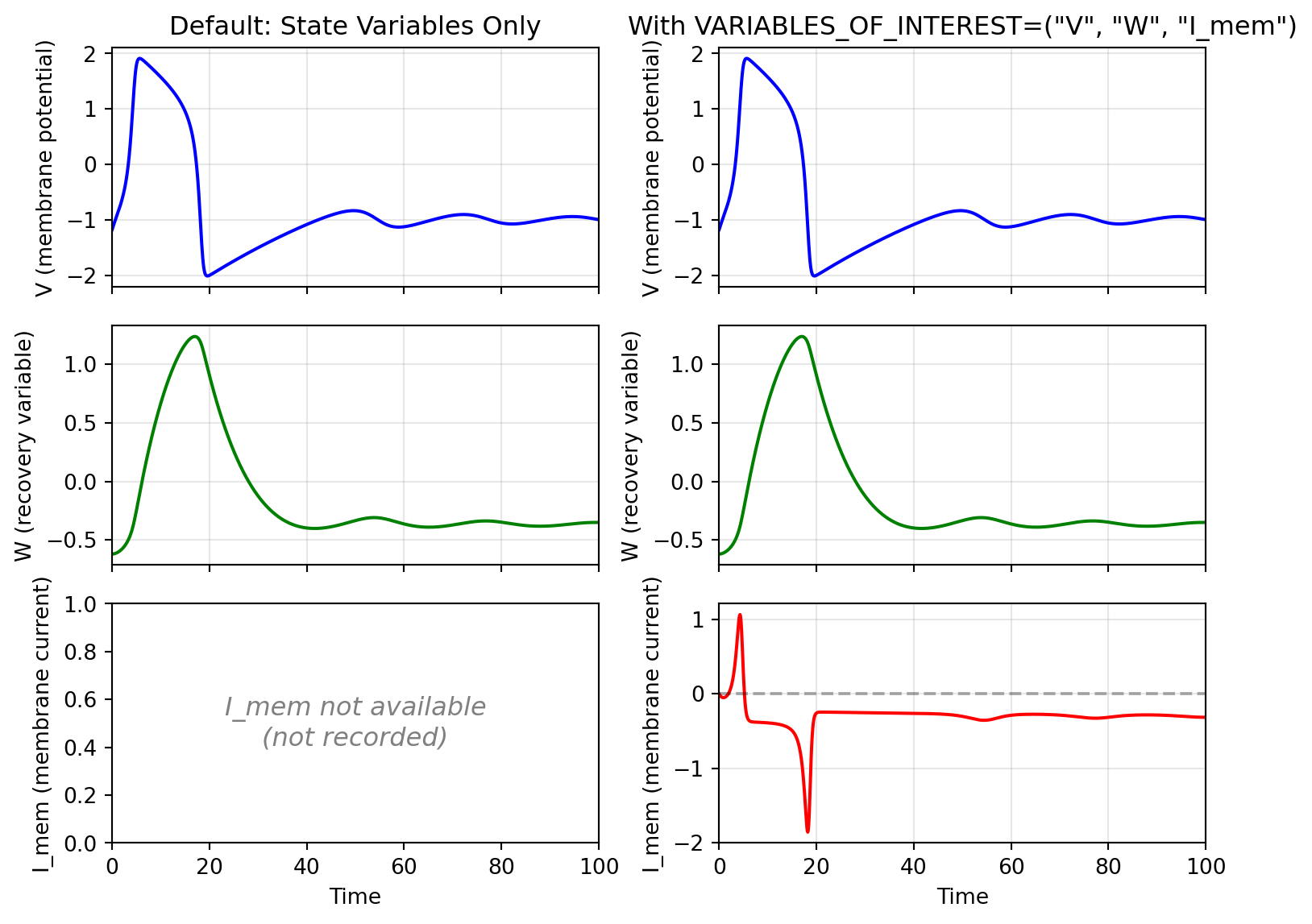
## Demonstrating Auxiliary Variables
Let's demonstrate how `VARIABLES_OF_INTEREST` controls what gets saved. We'll compare simulations with and without the auxiliary variable $I_{\text{mem}}$:
```{python}
from tvboptim.experimental.network_dynamics import solve
from tvboptim.experimental.network_dynamics.solvers import Euler

# Model without auxiliary in VOI (default)
fhn_default = FitzHughNagumo()

# Model with auxiliary in VOI
fhn_with_aux = FitzHughNagumo(
    VARIABLES_OF_INTEREST=('V', 'W', 'I_mem')
)

# Simulate both (bare dynamics — no network setup needed)
result_default = solve(fhn_default, Euler(), t0=0.0, t1=100.0, dt=0.1)
result_with_aux = solve(fhn_with_aux, Euler(), t0=0.0, t1=100.0, dt=0.1)

print(f"Default output shape: {result_default.ys.shape}  # [time, 2 states, nodes]")
print(f"With aux output shape: {result_with_aux.ys.shape}  # [time, 3 variables, nodes]")
```
```{python}
#| code-fold: true
#| code-summary: "Visualization"
import matplotlib.pyplot as plt

fig, axes = plt.subplots(3, 2, figsize=(8.1, 6.075), sharex=True)

# Left column: default (states only)
axes[0, 0].plot(result_default.ts, result_default.ys[:, 0, 0], 'b-')
axes[0, 0].set_ylabel('V (membrane potential)')
axes[0, 0].grid(True, alpha=0.3)
axes[0, 0].set_title('Default: State Variables Only')

axes[1, 0].plot(result_default.ts, result_default.ys[:, 1, 0], 'g-')
axes[1, 0].set_ylabel('W (recovery variable)')
axes[1, 0].grid(True, alpha=0.3)

axes[2, 0].text(0.5, 0.5, 'I_mem not available\n(not recorded)',
                ha='center', va='center', transform=axes[2, 0].transAxes,
                fontsize=12, style='italic', color='gray')
axes[2, 0].set_xlabel('Time')
axes[2, 0].set_ylabel('I_mem (membrane current)')
axes[2, 0].set_xlim(result_default.ts[0], result_default.ts[-1])

# Right column: with auxiliary
axes[0, 1].plot(result_with_aux.ts, result_with_aux.ys[:, 0, 0], 'b-')
axes[0, 1].set_ylabel('V (membrane potential)')
axes[0, 1].grid(True, alpha=0.3)
axes[0, 1].set_title('With VARIABLES_OF_INTEREST=("V", "W", "I_mem")')

axes[1, 1].plot(result_with_aux.ts, result_with_aux.ys[:, 1, 0], 'g-')
axes[1, 1].set_ylabel('W (recovery variable)')
axes[1, 1].grid(True, alpha=0.3)

axes[2, 1].plot(result_with_aux.ts, result_with_aux.ys[:, 2, 0], 'r-')
axes[2, 1].axhline(0, color='k', linestyle='--', alpha=0.3)
axes[2, 1].set_xlabel('Time')
axes[2, 1].set_ylabel('I_mem (membrane current)')
axes[2, 1].grid(True, alpha=0.3)

plt.tight_layout()
plt.show()
```
The membrane current $I_{\text{mem}}$ reveals the intrinsic dynamics: when positive, the membrane is driven toward depolarization; when negative, toward hyperpolarization. This auxiliary variable is essential for phase-plane analysis but increases memory usage, so include it in `VARIABLES_OF_INTEREST` only when needed.
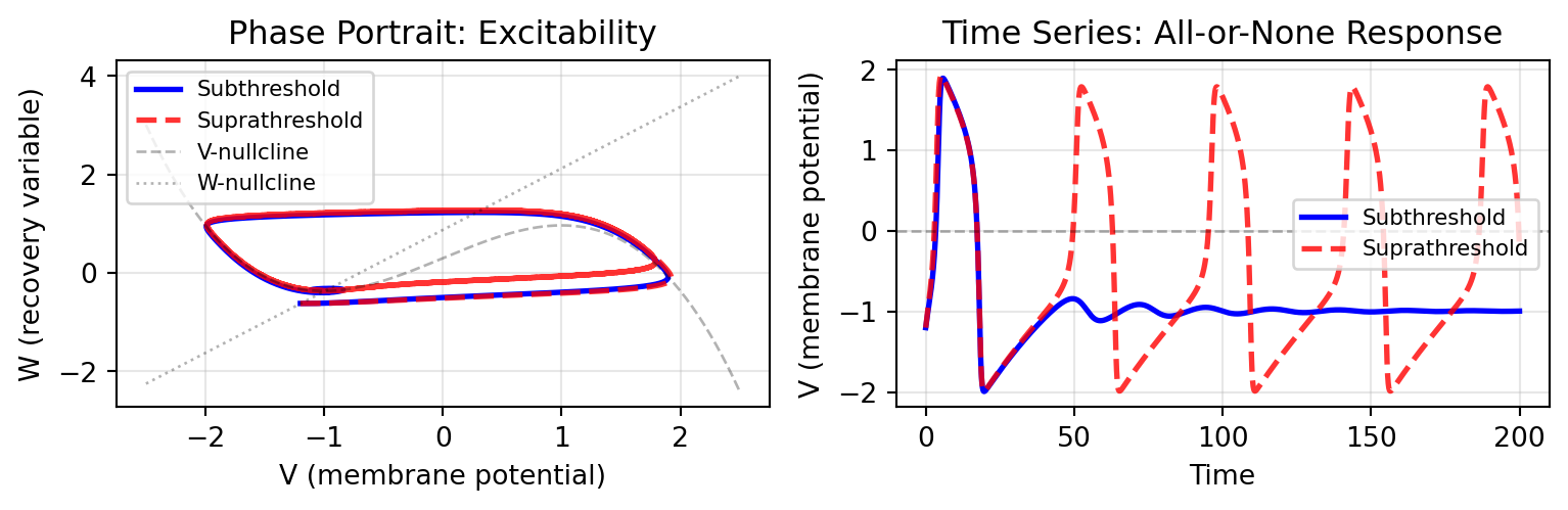
## Excitable Dynamics
Now let's demonstrate the characteristic excitable behavior, all-or-none responses to perturbations by increasing the background input $I$. Default parameters can be overridden at the creation of a dynamics object:
```{python}
# Initial states: small perturbation vs large perturbation

# Simulate both trajectories
times_sub, traj_sub = fhn.simulate(
    t0=0.0, t1=200.0, dt=0.1,
)

fhn_supra = FitzHughNagumo(I = 0.35) # Increased background input, default I = 0.3

times_sup, traj_sup = fhn_supra.simulate(
    t0=0.0, t1=200.0, dt=0.1,
)
```
```{python}
#| code-fold: true
#| code-summary: "Visualization"
fig, (ax1, ax2) = plt.subplots(1, 2, figsize=(8.1, 2.7))

# Phase portrait
ax1.plot(traj_sub[:, 0, 0], traj_sub[:, 1, 0], 'b-', label='Subthreshold', linewidth=2)
ax1.plot(traj_sup[:, 0, 0], traj_sup[:, 1, 0], 'r--', alpha = 0.8, label='Suprathreshold', linewidth=2)

# Nullclines for context
V_null = jnp.linspace(-2.5, 2.5, 200)
W_null_V = V_null - V_null**3 / 3.0 + fhn.params.I
W_null_W = (V_null + fhn.params.a) / fhn.params.b

ax1.plot(V_null, W_null_V, 'k--', alpha=0.3, linewidth=1, label='V-nullcline')
ax1.plot(V_null, W_null_W, 'k:', alpha=0.3, linewidth=1, label='W-nullcline')

ax1.set_xlabel('V (membrane potential)')
ax1.set_ylabel('W (recovery variable)')
ax1.legend(fontsize=8)
ax1.grid(True, alpha=0.3)
ax1.set_title('Phase Portrait: Excitability')

# Time series
ax2.plot(times_sub, traj_sub[:, 0, 0], 'b-', label='Subthreshold', linewidth=2)
ax2.plot(times_sup, traj_sup[:, 0, 0], 'r--', alpha = 0.8, label='Suprathreshold', linewidth=2)
ax2.axhline(0, color='k', linestyle='--', alpha=0.3, linewidth=1)
ax2.set_xlabel('Time')
ax2.set_ylabel('V (membrane potential)')
ax2.legend(fontsize=8)
ax2.grid(True, alpha=0.3)
ax2.set_title('Time Series: All-or-None Response')

plt.tight_layout()
plt.show()
```
The FitzHugh-Nagumo model exhibits classic excitable dynamics: subthreshold perturbations decay back to rest, while suprathreshold perturbations trigger a large-amplitude "spike" - the computational basis of neural coding.
# Available Dynamics Models
TVB-Optim includes several canonical models from computational neuroscience:
| Model | States | Type | Key Features | Use Cases |
|-------|--------|------|--------------|-----------|
| `Lorenz` | 3 | Chaotic | Butterfly attractor | Testing, demonstrations |
| `ReducedWongWang` | 1 | Neural mass | NMDA kinetics, decision-making | Resting-state fMRI, bistability |
| `JansenRit` | 6 | Neural mass | Cortical column, E/I balance | EEG/MEG modeling, oscillations |
| `Generic2dOscillator` | 2 | Oscillator | Flexible limit cycle | Rhythmic activity, alpha/beta |
| `WilsonCowan` | 2 | Neural mass | E/I populations | Population dynamics, pattern formation |
| `Epileptor` | 6 | Neural mass | Seizure dynamics | Epilepsy modeling, bifurcations |
| `Kuramoto` | 1 | Phase model | Synchronization | Phase coupling, oscillator networks |
See the [API Reference](../reference/index.qmd) for complete parameter descriptions and mathematical details.
# Summary
Dynamics models define the local temporal evolution at each network node:
- **Built-in models** cover common use cases from chaotic systems to biophysical neural masses
- **Auxiliary variables** must be explicitly included in `VARIABLES_OF_INTEREST` to be recorded
- **Custom dynamics** are straightforward to implement by subclassing `AbstractDynamics`
- **Parameter customization** enables model configuration without modifying source code (e.g., adjusting `I` in FitzHugh-Nagumo to control excitability)
- **Standalone methods** (`verify()`, `simulate()`, `plot()`) enable testing before network integration
The dynamics layer integrates seamlessly with coupling, graphs, and solvers to form complete brain network simulations. See [Coupling](coupling.qmd), [Graph](graph.qmd), and [Noise](noise.qmd) for building complete network models.
# References
::: {#refs}
:::