Network topology defines the structural connectivity between nodes - which regions connect to which, with what strength, and across what distance. The graph layer provides a unified interface for both dense and sparse connectivity representations.
The AbstractGraph Interface
All graph types inherit from AbstractGraph and provide these core properties:
from tvboptim.experimental.network_dynamics.graph import AbstractGraphclass MyGraph(AbstractGraph):@propertydef n_nodes(self) ->int:"""Number of nodes in the network."""pass@propertydef weights(self) -> jnp.ndarray:"""Weight matrix [n_nodes, n_nodes]."""pass@propertydef region_labels(self) -> Sequence[str]:"""Labels for each node (e.g., ['L.BSTS', 'R.MTG', ...])."""pass@propertydef sparsity(self) ->float:"""Fraction of non-zero connections (excluding diagonal)."""pass@propertydef symmetric(self) ->bool:"""Whether connectivity is symmetric (undirected)."""passdef verify(self, verbose: bool=True) ->bool:"""Check for valid structure (finite values, shape consistency)."""pass
The weights property returns a matrix compatible with JAX operations (@, jnp.matmul(), etc.) for both dense and sparse implementations.
Dense Graphs
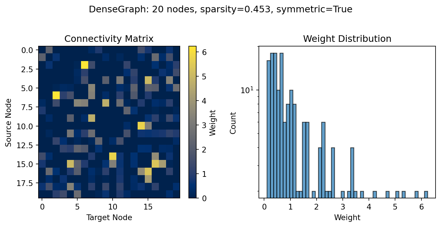
Dense graphs use standard JAX arrays to store the full connectivity matrix. This is the default choice for most brain networks.
The log-normal weight distribution captures the heavy-tailed structure observed in real brain connectivity, where most connections are weak but a few are very strong.
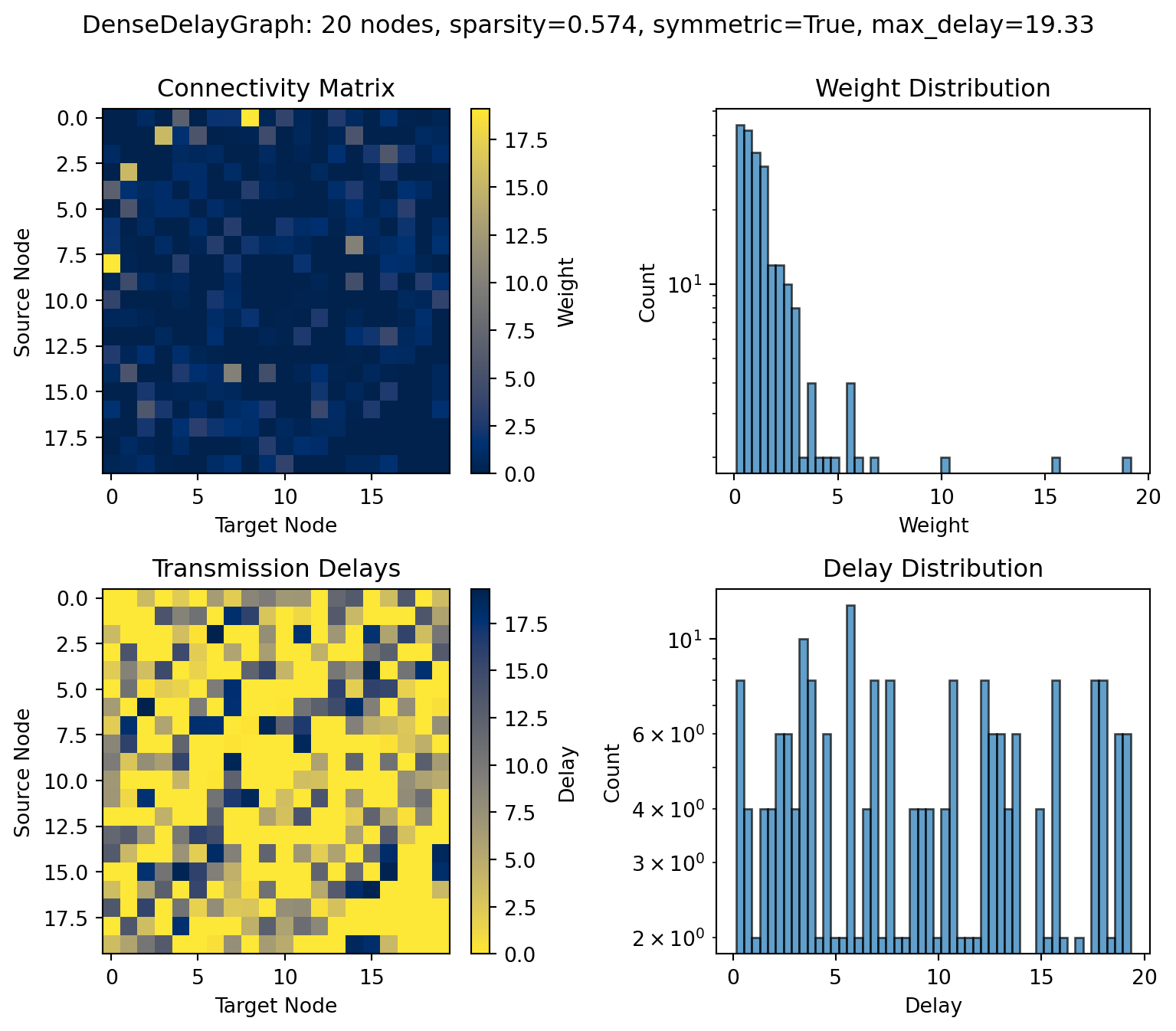
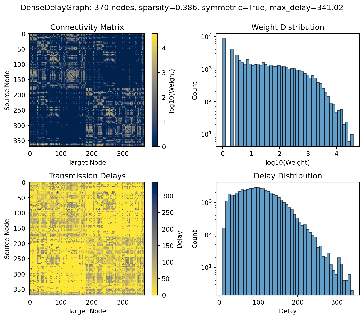
Delays: Distance-Dependent Transmission
Brain connectivity has finite transmission speeds - signals take time to propagate between regions. DenseDelayGraph models this with a delay matrix:
from tvboptim.experimental.network_dynamics.graph import DenseDelayGraph# Create graph with random delaysdelay_graph = DenseDelayGraph.random( n_nodes=20, sparsity=0.6, max_delay=20.0, # Maximum delay in ms delay_dist='uniform', key=key)print(delay_graph)
Delays are only meaningful for non-zero connections. The delay matrix shares the same sparsity pattern as the weight matrix.
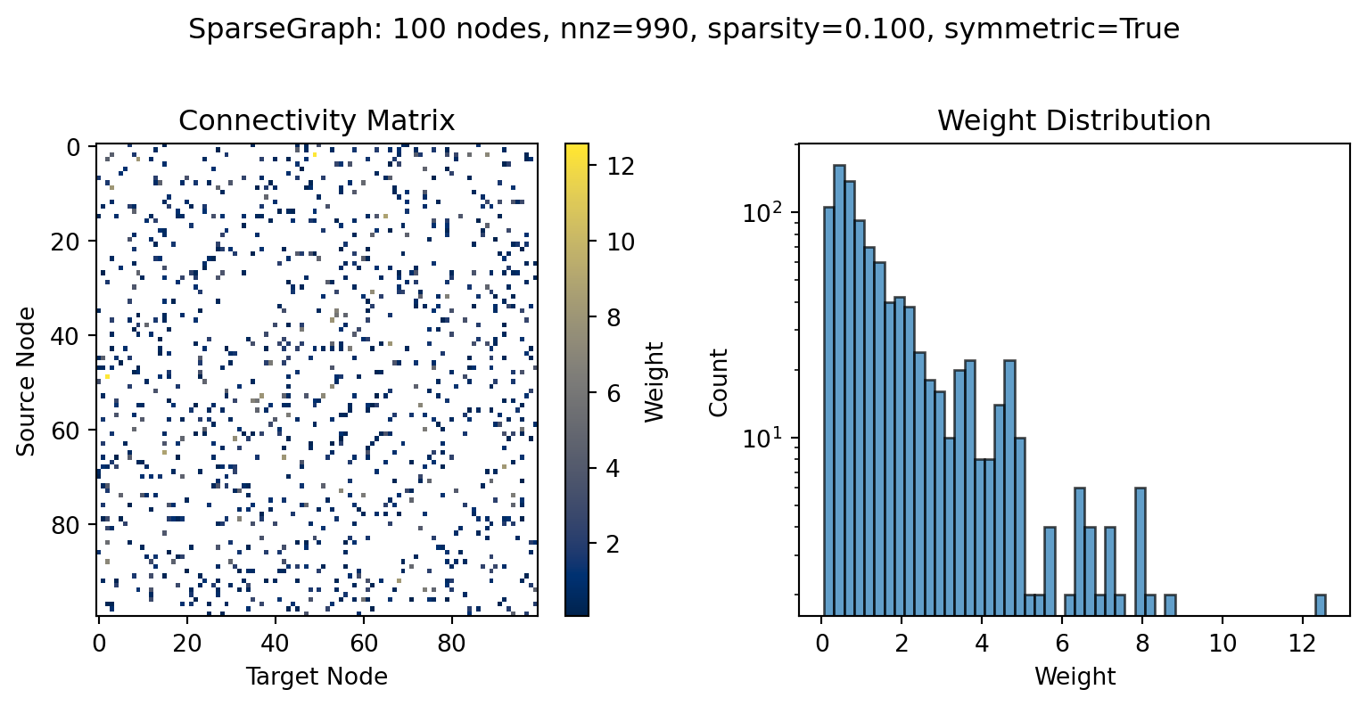
Sparse Graphs
For very large networks with extremely high sparsity (< 1% density), sparse storage can reduce memory usage. TVB-Optim uses JAX’s BCOO (Batched COO) format for sparse graphs. Such high sparsity is typical in surface-based simulations with tens of thousands of vertices.
WarningJAX Sparse Support is Experimental
JAX’s sparse matrix support is still experimental and has important performance characteristics:
Limited CPU performance: On CPU, JAX sparse operations are significantly slower than scipy’s optimized implementations
GPU advantage: On GPU, sparse operations can perform better than dense for very sparse matrices
Sparsity requirement: Performance benefits typically only appear for extremely sparse matrices (< 1% density)
Limited operations: Not all JAX operations support sparse arrays
For typical parcellated brain networks (50-500 regions with 30-90% density), dense graphs are strongly recommended.
When to Use Sparse Graphs
Use SparseGraph when:
Very large networks (> 10,000 nodes) with extreme sparsity (< 1% density)
Surface-based simulations with vertex-level connectivity
Running on GPU with memory constraints
Storage/serialization size is critical
Use DenseGraph when:
Parcellated brain networks (< 1,000 regions)
Density > 10%
Running on CPU
Performance is priority
Creating Sparse Graphs
from tvboptim.experimental.network_dynamics.graph import SparseGraph# From dense array (automatically sparsified)sparse_graph = SparseGraph(random_graph.weights, threshold=0.1)print(sparse_graph)print(f"Non-zero elements: {sparse_graph.nnz}")
---title: "Network Topology & Connectivity"format: html: code-fold: false toc: true toc-depth: 3 fig-width: 8 out-width: "100%"jupyter: python3execute: cache: true---Network topology defines the structural connectivity between nodes - which regions connect to which, with what strength, and across what distance. The graph layer provides a unified interface for both dense and sparse connectivity representations.# The AbstractGraph InterfaceAll graph types inherit from `AbstractGraph` and provide these core properties:```pythonfrom tvboptim.experimental.network_dynamics.graph import AbstractGraphclass MyGraph(AbstractGraph):@propertydef n_nodes(self) ->int:"""Number of nodes in the network."""pass@propertydef weights(self) -> jnp.ndarray:"""Weight matrix [n_nodes, n_nodes]."""pass@propertydef region_labels(self) -> Sequence[str]:"""Labels for each node (e.g., ['L.BSTS', 'R.MTG', ...])."""pass@propertydef sparsity(self) ->float:"""Fraction of non-zero connections (excluding diagonal)."""pass@propertydef symmetric(self) ->bool:"""Whether connectivity is symmetric (undirected)."""passdef verify(self, verbose: bool=True) ->bool:"""Check for valid structure (finite values, shape consistency)."""pass```The `weights` property returns a matrix compatible with JAX operations (`@`, `jnp.matmul()`, etc.) for both dense and sparse implementations.# Dense GraphsDense graphs use standard JAX arrays to store the full connectivity matrix. This is the default choice for most brain networks.## Creating Dense Graphs```{python}import jax.numpy as jnpfrom tvboptim.experimental.network_dynamics.graph import DenseGraph# From connectivity matrixweights = jnp.array([ [0.0, 0.5, 0.2], [0.5, 0.0, 0.8], [0.2, 0.8, 0.0]])graph = DenseGraph(weights)graph.verify()```The graph automatically detects properties like symmetry and computes sparsity:```{python}print(f"Nodes: {graph.n_nodes}")print(f"Sparsity: {graph.sparsity:.3f}")print(f"Symmetric: {graph.symmetric}")print(f"Region labels: {graph.region_labels}")```## Random Graph GenerationThe `.random()` classmethod creates synthetic networks with brain-like connectivity statistics:```{python}import jax# Create random graph with 50% densitykey = jax.random.key(42)random_graph = DenseGraph.random( n_nodes=20, sparsity=0.5, # 50% of connections present symmetric=True, # Undirected connectivity weight_dist='lognormal', # Heavy-tailed weight distribution key=key)print(random_graph)``````{python}random_graph.plot(figsize=(8.1, 4));```The log-normal weight distribution captures the heavy-tailed structure observed in real brain connectivity, where most connections are weak but a few are very strong.## Delays: Distance-Dependent TransmissionBrain connectivity has finite transmission speeds - signals take time to propagate between regions. `DenseDelayGraph` models this with a delay matrix:```{python}from tvboptim.experimental.network_dynamics.graph import DenseDelayGraph# Create graph with random delaysdelay_graph = DenseDelayGraph.random( n_nodes=20, sparsity=0.6, max_delay=20.0, # Maximum delay in ms delay_dist='uniform', key=key)print(delay_graph)``````{python}delay_graph.plot(figsize=(8.1, 7));```Delays are only meaningful for non-zero connections. The delay matrix shares the same sparsity pattern as the weight matrix.# Sparse GraphsFor very large networks with extremely high sparsity (< 1% density), sparse storage can reduce memory usage. TVB-Optim uses JAX's [BCOO (Batched COO) format](https://jax.readthedocs.io/en/latest/jax.experimental.sparse.html) for sparse graphs. Such high sparsity is typical in surface-based simulations with tens of thousands of vertices.::: {.callout-warning}## JAX Sparse Support is ExperimentalJAX's sparse matrix support is still experimental and has important performance characteristics:- **Limited CPU performance**: On CPU, JAX sparse operations are significantly slower than scipy's optimized implementations- **GPU advantage**: On GPU, sparse operations can perform better than dense for very sparse matrices- **Sparsity requirement**: Performance benefits typically only appear for extremely sparse matrices (< 1% density)- **Limited operations**: Not all JAX operations support sparse arraysFor typical parcellated brain networks (50-500 regions with 30-90% density), **dense graphs are strongly recommended**.:::## When to Use Sparse GraphsUse `SparseGraph` when:- Very large networks (> 10,000 nodes) with extreme sparsity (< 1% density)- Surface-based simulations with vertex-level connectivity- Running on GPU with memory constraints- Storage/serialization size is criticalUse `DenseGraph` when:- Parcellated brain networks (< 1,000 regions)- Density > 10%- Running on CPU- Performance is priority## Creating Sparse Graphs```{python}from tvboptim.experimental.network_dynamics.graph import SparseGraph# From dense array (automatically sparsified)sparse_graph = SparseGraph(random_graph.weights, threshold=0.1)print(sparse_graph)print(f"Non-zero elements: {sparse_graph.nnz}")``````{python}# Convert dense to sparsesparse_from_dense = SparseGraph.from_dense(random_graph, threshold=0.1)# Create random sparse graphsparse_random = SparseGraph.random( n_nodes=100, sparsity=0.1, # Only 10% density key=key)sparse_random.plot(figsize=(8.1, 4));```The BCOO format stores only non-zero elements, making it memory-efficient for sparse connectivity.# Example Connectivity DataTVB-Optim includes example structural connectivity datasets useful for testing and development:- **`dk_average`**: Desikan-Killiany atlas, 84 cortical regions, averaged across subjects- **`dTOR`**: Virtual DBS dataset with Glasser parcellation, 370 regions (cortex + subcortex + striatum)## "dk_average"```{python}from tvboptim.data import load_structural_connectivity# Load dk_average datasetweights_dk, lengths_dk, labels_dk = load_structural_connectivity("dk_average")print(f"Regions: {len(labels_dk)}")print(f"Example labels: {labels_dk[:3]}")print(f"Sparsity: {jnp.count_nonzero(weights_dk) / (weights_dk.shape[0] * (weights_dk.shape[0] -1)):.3f}")``````{python}# Create graph and plotgraph_dk = DenseDelayGraph(weights_dk, lengths_dk, region_labels=labels_dk)graph_dk.plot(log_scale_weights=True, figsize=(8.1, 7));```## "dTOR"```{python}# Load dTOR datasetweights_dtor, lengths_dtor, labels_dtor = load_structural_connectivity("dTOR")print(f"Regions: {len(labels_dtor)}")print(f"Example labels: {labels_dtor[:3]}")print(f"Sparsity: {jnp.count_nonzero(weights_dtor) / (weights_dtor.shape[0] * (weights_dtor.shape[0] -1)):.3f}")``````{python}# Create graph and plotgraph_dtor = DenseDelayGraph(weights_dtor, lengths_dtor, region_labels=labels_dtor)graph_dtor.plot(log_scale_weights=True, figsize=(8.1, 7));```