---
title: "Extending Coupling 2: Short-Term Plasticity"
subtitle: "Giving a Connection Its Own Per-Edge State"
format:
html:
code-fold: false
toc: true
toc-depth: 3
fig-width: 8
out-width: "100%"
jupyter: python3
execute:
cache: true
---
Try this notebook interactively:
[Download .ipynb](https://github.com/virtual-twin/tvboptim/blob/main/docs/advanced/stateful_edge_coupling.ipynb){.btn .btn-primary download="stateful_edge_coupling.ipynb"}
[Download .qmd](stateful_edge_coupling.qmd){.btn .btn-secondary download="stateful_edge_coupling.qmd"}
[Open in Colab](https://colab.research.google.com/github/virtual-twin/tvboptim/blob/main/docs/advanced/stateful_edge_coupling.ipynb){.btn .btn-warning target="_blank"}
# Introduction
Every coupling shipped with tvboptim is memoryless in the connection: what it transmits is a function of the **current node state**. `LinearCoupling` transmits $S_j$, `DelayedKuramotoCoupling` transmits $\sin(\theta_j(t - \tau_{ij}) - \theta_i)$, and a custom `pre()` transmits any pointwise transform of the selected states.
Short-term synaptic plasticity breaks that assumption. A depressing synapse transmits less when it has been driven recently, so transmission depends on presynaptic activity **and** on a hidden variable owned by the connection. That variable is **per edge**: node $j$ can project along one depressed and one rested pathway at the same time, which rules out storing it as node state.
This notebook builds such a coupling from the general interface: `prepare()`, `precompute()`, `compute()` and `update_state()`. The coupling allocates edge-shaped state and carries it through the solver's scan. Dynamics model, solver and network remain untouched, and the same class then supports a mixed population of depressing and facilitating synapses without further code.
```{python}
#| output: false
#| echo: false
# Install dependencies if running in Google Colab
try:
import google.colab
print("Running in Google Colab - installing dependencies...")
!pip install -q tvboptim
print("✓ Dependencies installed!")
except ImportError:
pass # Not in Colab, assume dependencies are available
```
```{python}
#| code-fold: true
#| code-summary: "Environment Setup and Imports"
import copy

import jax
import jax.numpy as jnp
import numpy as np
import matplotlib.pyplot as plt

from tvboptim.types import Space, LogGridAxis
from tvboptim.execution import ParallelExecution
from tvboptim.experimental.network_dynamics import Bunch, Network, solve, prepare
from tvboptim.experimental.network_dynamics.coupling import (
    AbstractCoupling,
    LinearCoupling,
)
from tvboptim.experimental.network_dynamics.dynamics.tvb import WilsonCowan
from tvboptim.experimental.network_dynamics.graph import DenseGraph, SparseGraph
from tvboptim.experimental.network_dynamics.noise import AdditiveNoise
from tvboptim.experimental.network_dynamics.solvers import Heun

jax.config.update("jax_enable_x64", True)

PLASTIC, STATIC = "steelblue", "coral"
```
# The Model
The Tsodyks-Markram description gives each connection a fraction of available resources $x$, released with probability $u$ on every presynaptic event:
$$
\begin{aligned}
\frac{dx_{ij}}{dt} &= \frac{1 - x_{ij}}{\tau_d} - u_{ij} x_{ij} r_j \\
\frac{du_{ij}}{dt} &= \frac{U - u_{ij}}{\tau_f} + U (1 - u_{ij}) r_j
\end{aligned}
$$
Drive depletes resources, which recover with time constant $\tau_d$ (**depression**), and raises release probability above its baseline $U$, from which it decays with $\tau_f$ (**facilitation**). The presynaptic rate is $r_j = \nu E_j$, and what the connection transmits is proportional to the product $u x$:
$$
c_i = G \sum_j w_{ij} \, \frac{u_{ij} x_{ij}}{U} \, E_j
$$
Normalising by $U$ sets the synaptic gain $u x / U$ to 1 for a rested synapse, so $G$ keeps the meaning it has in a `LinearCoupling` on the same graph. The comparison below depends on that.
# Mapping to the Coupling API
Most custom couplings subclass `InstantaneousCoupling` or `DelayedCoupling` and override only `pre()` or `post()`, because the framework's select, transform, aggregate, transform sequence already describes them. This one does not fit that sequence: the transmitted signal depends on a carry that `pre()` never sees. `AbstractCoupling` is the right base precisely in that case, at the cost of implementing the four phases directly.
| Phase | When it runs | What it does here |
|---|---|---|
| `prepare()` | Once, outside JIT | Resolves state indices and the edge layout, allocates the initial $x$ and $u$ |
| `precompute()` | Once per forward pass, inside JIT | Broadcasts the live plasticity parameters to edge shape |
| `compute()` | Every step (or every stage) | Multiplies presynaptic activity by the current synaptic gain and reduces onto targets |
| `update_state()` | Every step, after integration | Advances $x$ and $u$ with the new presynaptic activity |
Two points deserve emphasis. `precompute()` is not an optimisation here, it is the only route by which parameters reach the update: the solver calls `update_state(coupling_data, coupling_state, new_state)`, which has no `params` argument, and `precompute()` is the one hook that sees both the live parameters and `coupling_data`. Writing $\tau_d$, $\tau_f$ and $U$ there once per forward pass keeps them ordinary traced leaves, hence differentiable and sweepable. Everything static belongs in `prepare()` instead, the edge index maps included: graph topology is fixed for the life of a prepared solve, so resolving it per forward pass would be wasted work.
`coupling_state`, in turn, is a scan carry and may hold anything of fixed shape. `DelayedCoupling` uses it for a history buffer; here it holds two edge-shaped arrays.
# Implementation
```{python}
class ShortTermPlasticityCoupling(AbstractCoupling):
    """Tsodyks-Markram short-term plasticity carried by the connection itself.

    Each edge owns a depression variable ``x`` and a facilitation variable
    ``u``, driven by the presynaptic rate ``nu * E_j``. What crosses the
    connection is ``G * w_ij * (u_ij * x_ij / U) * E_j``, so the synaptic
    gain ``u * x / U`` is 1 for a rested synapse.
    """

    N_OUTPUT_STATES = 1
    DEFAULT_PARAMS = Bunch(G=1.0, tau_d=200.0, tau_f=600.0, U=0.2, nu=1.0)

    def _layout(self, graph):
        """Edge-array shape and index maps, for dense and sparse graphs alike."""
        if isinstance(graph, SparseGraph):
            edges = graph.edge_indices
            return Bunch(
                shape=(graph.nnz,),
                target_e=edges[:, 0],
                source_e=edges[:, 1],
                n_target=graph.weights.shape[0],
                is_sparse=True,
            )

        n_target, n_source = graph.weights.shape
        return Bunch(
            shape=(n_target, n_source),
            target_e=None,
            source_e=None,
            n_target=n_target,
            is_sparse=False,
        )

    def prepare(self, network, dt, t0, t1):
        """Static setup and the initial carry."""
        del t0, t1
        layout = self._layout(network.graph)
        dtype = network.initial_state.dtype

        # Topology is fixed for the life of a prepared solve, so the index
        # maps are resolved here rather than once per forward pass.
        coupling_data = Bunch(
            incoming_indices=network.dynamics.name_to_index(self.SOURCE_STATE_NAMES),
            local_indices=network.dynamics.name_to_index(self.LOCAL_STATE_NAMES),
            dt=dt,
            edge_shape=layout.shape,
            target_e=layout.target_e,
            source_e=layout.source_e,
            n_target=layout.n_target,
            is_sparse=layout.is_sparse,
        )

        # Synapses start rested: full resources, baseline release probability.
        coupling_state = Bunch(
            x=jnp.ones(layout.shape, dtype=dtype),
            u=jnp.broadcast_to(jnp.asarray(self.params.U), layout.shape).astype(dtype),
        )
        return coupling_data, coupling_state

    def precompute(self, coupling_data, params, graph):
        """Live plasticity parameters to edge shape, once per forward pass."""
        del graph
        coupling_data = coupling_data.copy()
        shape = coupling_data.edge_shape

        # Broadcasting accepts a scalar or a per-edge array, so heterogeneous
        # synapse populations need no change below this line.
        coupling_data.stp = Bunch(
            tau_d=jnp.broadcast_to(jnp.asarray(params.tau_d), shape),
            tau_f=jnp.broadcast_to(jnp.asarray(params.tau_f), shape),
            U=jnp.broadcast_to(jnp.asarray(params.U), shape),
            nu=jnp.asarray(params.nu),
        )
        return coupling_data

    def _source_activity(self, network_state, coupling_data):
        """Presynaptic activity laid out per edge."""
        activity = network_state[coupling_data.incoming_indices][0]
        if coupling_data.is_sparse:
            return activity[coupling_data.source_e]
        return jnp.broadcast_to(activity[None, :], coupling_data.edge_shape)

    def _reduce(self, released, coupling_data, graph):
        """Sum weighted edge messages onto their target nodes."""
        if coupling_data.is_sparse:
            return jax.ops.segment_sum(
                released * graph.weights.data,
                coupling_data.target_e,
                num_segments=coupling_data.n_target,
            )
        return jnp.sum(released * graph.weights, axis=-1)

    def compute(self, t, state, coupling_data, coupling_state, params, graph):
        """The transmitted signal: gain from the carry, activity from the state."""
        del t
        gain = coupling_state.u * coupling_state.x / coupling_data.stp.U
        activity = self._source_activity(state, coupling_data)
        return (params.G * self._reduce(gain * activity, coupling_data, graph))[None, :]

    def update_state(self, coupling_data, coupling_state, new_state):
        """Advance the synapses with the activity the step just produced."""
        stp, dt = coupling_data.stp, coupling_data.dt
        rate = stp.nu * self._source_activity(new_state, coupling_data)
        x, u = coupling_state.x, coupling_state.u

        dx = (1.0 - x) / stp.tau_d - u * x * rate
        du = (stp.U - u) / stp.tau_f + stp.U * (1.0 - u) * rate
        return Bunch(x=x + dt * dx, u=u + dt * du)

    def describe(self):
        """How the network printer should render this coupling."""
        return {
            "network_form": "G * Σⱼ wᵢⱼ * (uᵢⱼ xᵢⱼ / U) * Eⱼ",
            "pre_form": None,
            "post_form": None,
        }
```
Note what the class does **not** contain: solver code, an explicit scan, manual carry threading, a bespoke parameter container. The edge state rides in the carry the framework already maintains, and the plasticity time constants are ordinary parameter leaves.
# Building the Network
Wilson-Cowan is a convenient substrate: `E` is a normalised excitatory activity, and the model already declares a one-dimensional long-range input onto the excitatory population. The parameters below sit in a limit-cycle regime, and weak additive noise on `E` keeps the nodes off a common orbit, so that the synapses see irregular rather than strictly periodic drive.
```{python}
WC_OSCILLATORY = dict(
    c_ee=16.0, c_ei=12.0, c_ie=15.0, c_ii=3.0,
    a_e=1.3, b_e=4.0, a_i=2.0, b_i=3.7,
    P=1.25, tau_e=8.0, tau_i=8.0,
)

n_nodes = 20
random_graph = DenseGraph.random(n_nodes, density=0.4, key=jax.random.key(3))

# Row-normalise so that G is the total long-range drive per node.
graph = DenseGraph(
    weights=random_graph.weights / jnp.sum(random_graph.weights, axis=1, keepdims=True)
)
noise = AdditiveNoise(apply_to="E", sigma=0.01, key=jax.random.key(7))

t0, t1, dt = 0.0, 1500.0, 0.1


def build(coupling, g=graph, n=noise):
    """Wilson-Cowan network driven through a single long-range coupling."""
    return Network(WilsonCowan(**WC_OSCILLATORY), {"delayed": coupling}, g, noise=n)


def stp(**kwargs):
    return ShortTermPlasticityCoupling(source="E", G=8.0, **kwargs)


network = build(stp())
result = solve(network, Heun(), t0=t0, t1=t1, dt=dt)
print(f"Result shape: {result.ys.shape}")
```
::: {.callout-note}
`delayed` is the name Wilson-Cowan gives its long-range coupling channel. The name declares a channel in the dynamics model, not a property of the coupling attached to it, so an instantaneous coupling may serve it.
:::
The custom `describe()` is what the network printer renders for this coupling:
```{python}
#| code-fold: true
#| code-summary: "Network inspection"
from tvboptim.experimental.network_dynamics.utils.printer import CouplingDescriptor

print(CouplingDescriptor(network.coupling["delayed"], network).describe()["network_form"])
```
## Dense and Sparse Agree
`_layout()` is the only place that knows which graph representation is in use, so if it is correct the two paths describe the same simulation. Noise is switched off here so that any residual difference is purely arithmetic.
```{python}
result_dense = solve(build(stp(), n=None), Heun(), t0=t0, t1=t1, dt=dt)
result_sparse = solve(
    build(stp(), SparseGraph.from_dense(graph), n=None), Heun(), t0=t0, t1=t1, dt=dt
)

gap = jnp.max(jnp.abs(jnp.asarray(result_dense.ys) - jnp.asarray(result_sparse.ys)))
print(f"dense vs sparse, max |difference| over the trajectory: {gap:.2e}")
```
# What the Plasticity Does
With the gain normalised, `LinearCoupling` at the same `G` is the natural control: same network, same drive, static synapses. Because `G` is an ordinary leaf in `config`, the comparison runs as a native sweep rather than a Python loop over rebuilt networks.
```{python}
GAIN_AXIS = (1.0, 16.0, 5)  # low, high, n
gains = np.asarray(LogGridAxis(*GAIN_AXIS).generate_values())


def sweep_gain(coupling):
    """Mean level and oscillation amplitude of E over the last 500 ms, across G."""
    solve_fn, config = prepare(build(coupling), Heun(), t0=t0, t1=t1, dt=dt)
    config = copy.deepcopy(config)
    config.coupling.delayed.G = LogGridAxis(*GAIN_AXIS)

    def summarize(cfg):
        tail = solve_fn(cfg).ys[-5000:, 0]
        return jnp.stack([tail.mean(), jnp.mean(tail.max(0) - tail.min(0))])

    space = Space(config, mode="product")
    return np.asarray(ParallelExecution(summarize, space, n_vmap=len(gains)).run())


plastic = sweep_gain(stp())
static = sweep_gain(LinearCoupling(source="E", G=8.0))

for G, p, s in zip(gains, plastic, static):
    print(f"G={G:5.1f}   plastic: mean={p[0]:.3f} amp={p[1]:.3f}"
          f"   static: mean={s[0]:.3f} amp={s[1]:.3f}")
```
```{python}
#| code-fold: true
#| code-summary: "Visualization: Gain Control"
ys_lin = jnp.asarray(solve(
    build(LinearCoupling(source="E", G=8.0)), Heun(), t0=t0, t1=t1, dt=dt
).ys)

window = slice(-4000, None)
ts = np.asarray(result.ts)[window]

fig, axes = plt.subplot_mosaic("ab\ncc", figsize=(9, 5.5), dpi=200)

for ax, col, name in ((axes["a"], 0, "Mean E"), (axes["b"], 1, "Amplitude of E")):
    ax.plot(gains, static[:, col], "o-", color=STATIC, label="static synapses")
    ax.plot(gains, plastic[:, col], "o-", color=PLASTIC, label="plastic synapses")
    ax.set_xscale("log", base=2)
    ax.set_xlabel("Long-range gain G")
    ax.set_ylabel(name)
    ax.legend(fontsize=8)
    ax.grid(True, alpha=0.3)

axes["a"].set_title("Operating point")
axes["b"].set_title("Limit cycle")

axes["c"].plot(ts, np.asarray(ys_lin[window, 0, :5]), color=STATIC, alpha=0.8, lw=1)
axes["c"].plot(ts, np.asarray(result.ys[window, 0, :5]), color=PLASTIC, alpha=0.8, lw=1)
axes["c"].set_xlabel("Time [ms]")
axes["c"].set_ylabel("E")
axes["c"].set_title("G = 8: static synapses saturate, plastic synapses keep oscillating")
axes["c"].grid(True, alpha=0.3)

plt.tight_layout()
plt.show()
```
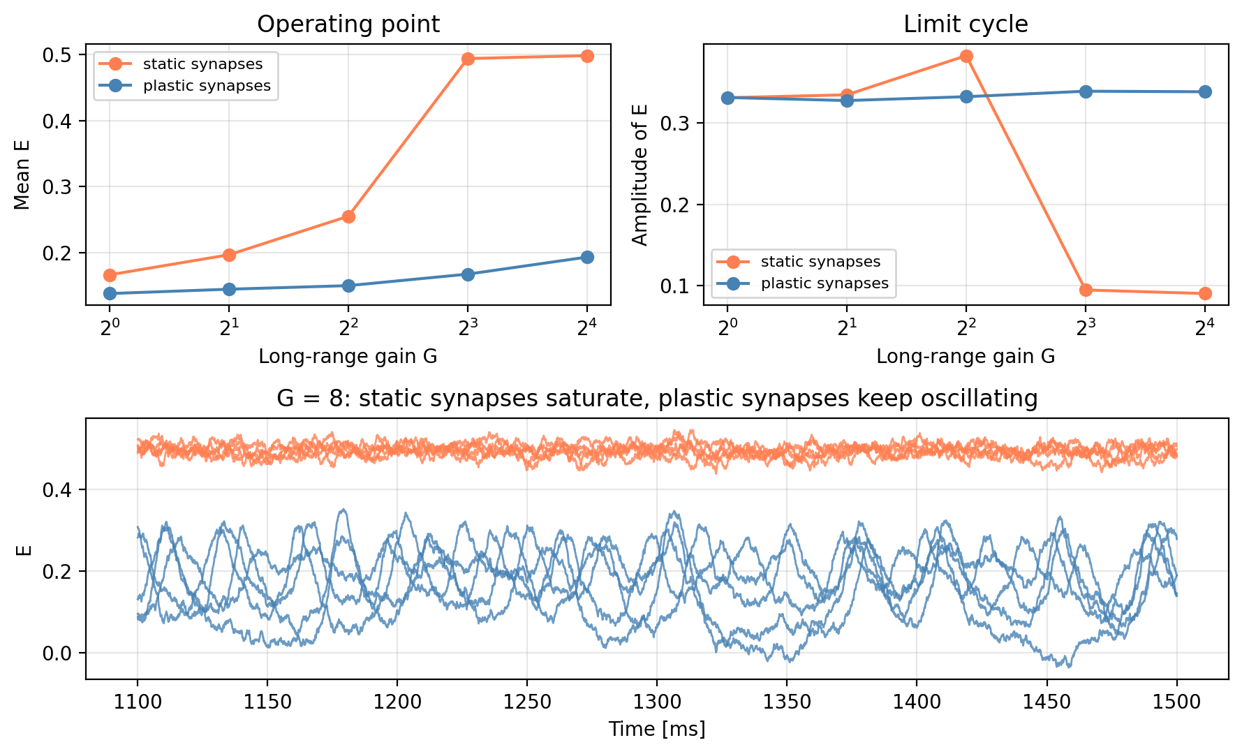
The static network follows its drive: as `G` grows, the operating point climbs until the excitatory population saturates and the limit cycle disappears. The plastic network holds its operating point across the same range, since stronger drive depletes its synapses further, and it still oscillates where the static network has fallen silent.
# Heterogeneous Synapses
Real projections are not a single population. Cortical synapses range from strongly depressing (high release probability, little facilitation) to facilitating (low release probability, long $\tau_f$), and the type an axon forms can depend on the target it reaches. That is an edge property. Since `precompute()` already broadcasts per-edge arrays, a mixed population costs no more than the parameter arrays themselves.
```{python}
facilitating = jax.random.bernoulli(jax.random.key(11), 0.5, (n_nodes, n_nodes))

heterogeneous = stp(
    tau_d=jnp.where(facilitating, 80.0, 50.0),
    tau_f=jnp.where(facilitating, 800.0, 50.0),
    U=jnp.where(facilitating, 0.1, 0.5),
)

network_het = build(heterogeneous)
result_het = solve(network_het, Heun(), t0=t0, t1=t1, dt=dt)
```
`result.ys` records the dynamics state. The synaptic variables live in the coupling carry, which the solver threads through the scan without emitting. They remain recoverable: `update_state()` is called once per step with the state that step produced, which is precisely what `result.ys` holds, so scanning the coupling's own `update_state()` over the recorded trajectory replays the carry step for step.
```{python}
data_dict, state_dict = network_het.prepare(dt=dt, t0=t0, t1=t1)
edge_data = heterogeneous.precompute(
    data_dict["delayed"], heterogeneous.params, network_het.graph
)


def replay(carry, network_state):
    carry = heterogeneous.update_state(edge_data, carry, network_state)
    return carry, carry.u * carry.x / edge_data.stp.U


_, gain_trace = jax.lax.scan(replay, state_dict["delayed"], jnp.asarray(result_het.ys))
print(f"Synaptic gain trace: {gain_trace.shape}  (time, target, source)")
print(f"Gain range across all edges: {gain_trace.min():.3f} to {gain_trace.max():.3f}")
```
::: {.callout-note}
The replay relies on the default `VARIABLES_OF_INTEREST`, which records the full integrated state in declaration order, the layout `update_state()` indexes into. A model that records only a subset, or that interleaves auxiliary variables, needs the recording restored to that layout first.
:::
```{python}
#| code-fold: true
#| code-summary: "Visualization: Two Synapse Types on the Same Axon"
exists = np.asarray(graph.weights) > 0
is_fac = np.asarray(facilitating)

# Source nodes that project through both a facilitating and a depressing edge.
pairs = [
    (j, np.flatnonzero(exists[:, j] & is_fac[:, j])[0],
     np.flatnonzero(exists[:, j] & ~is_fac[:, j])[0])
    for j in range(n_nodes)
    if (exists[:, j] & is_fac[:, j]).any() and (exists[:, j] & ~is_fac[:, j]).any()
][:3]

FAC, DEP = "mediumseagreen", "indianred"
fig, axes = plt.subplots(2, 1, figsize=(8, 4.5), dpi=200, sharex=True)

for j, i_fac, i_dep in pairs:
    axes[0].plot(ts, np.asarray(gain_trace[window, i_fac, j]), color=FAC, lw=1, alpha=0.8)
    axes[0].plot(ts, np.asarray(gain_trace[window, i_dep, j]), color=DEP, lw=1, alpha=0.8)
    axes[1].plot(ts, np.asarray(result_het.ys[window, 0, j]), lw=1, alpha=0.8)

axes[0].axhline(1.0, color="black", ls="--", lw=0.8, alpha=0.5)
axes[0].plot([], [], color=FAC, label="facilitating")
axes[0].plot([], [], color=DEP, label="depressing")
axes[0].set_ylabel("Synaptic gain u·x / U")
axes[0].set_title("Three source nodes, two synapse types each")
axes[0].legend(fontsize=8)
axes[0].grid(True, alpha=0.3)

axes[1].set_xlabel("Time [ms]")
axes[1].set_ylabel("Presynaptic E")
axes[1].set_title("Activity of those source nodes, shared by both synapse types")
axes[1].grid(True, alpha=0.3)

plt.tight_layout()
plt.show()
```
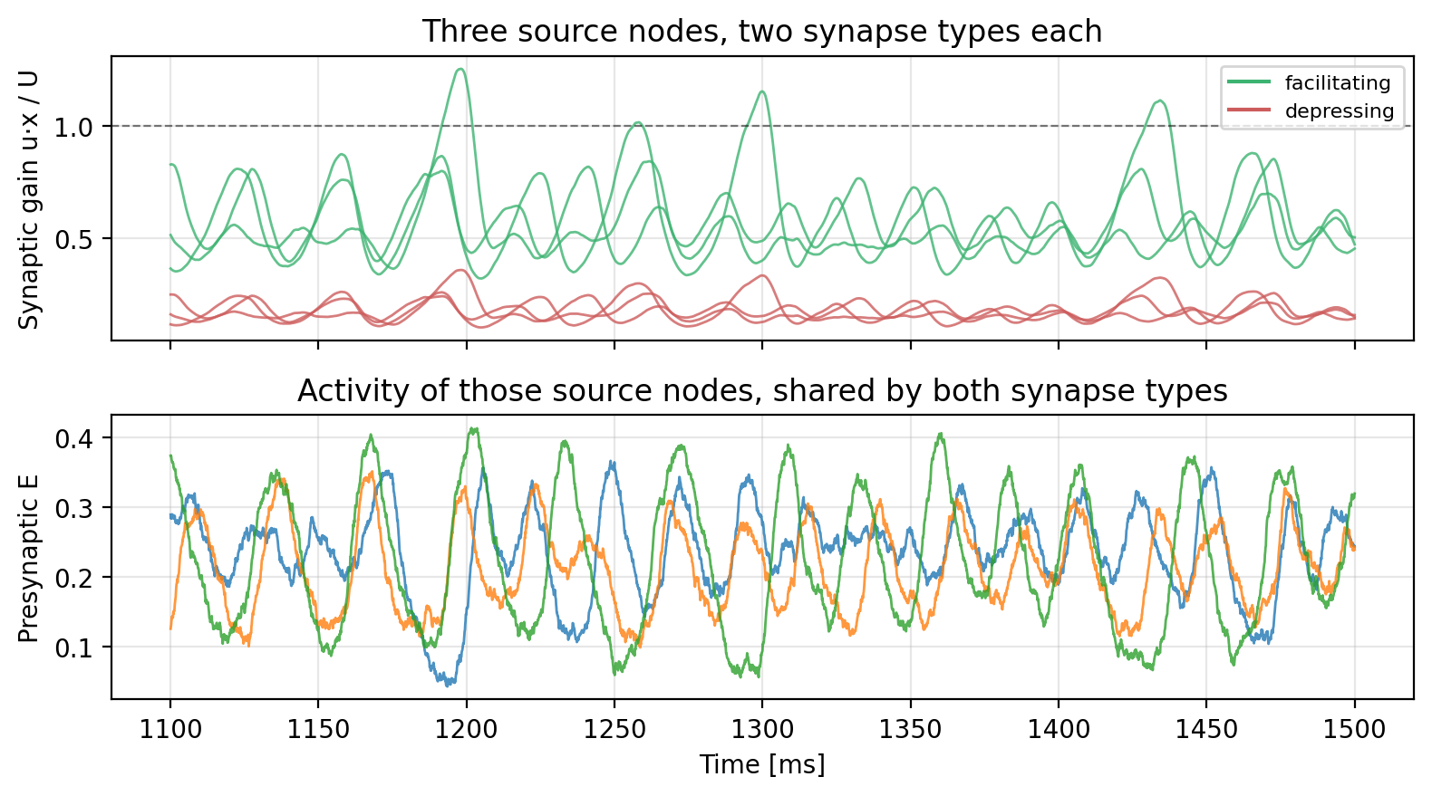
Each pair of traces leaves the **same** source node and sees the same bursts, yet the two respond in opposite directions: the facilitating edge climbs with each burst, exceeding the rested level on the strongest ones, while the depressing edge stays well below it and recovers little in between. No part of that difference can be expressed as node state.
# Accuracy and Limits
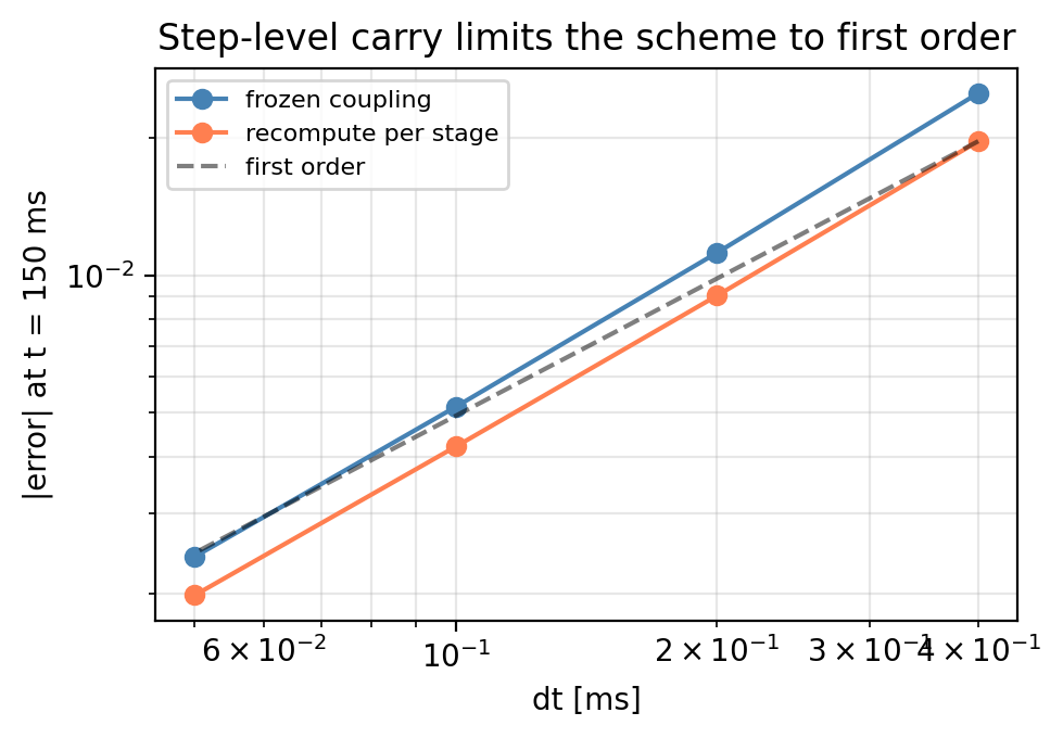
The synaptic state is a **step-level** carry: the solver computes it once per step in `update_state()`, after the dynamics step has completed, and holds it fixed across the stages of the next step. `DelayedCoupling` treats its history buffer the same way, with the same consequence: whatever the order of the outer solver, the coupling's own state contributes a first-order error.
The reference below is the same scheme at a step size far smaller than any tested one, with noise switched off so that the comparison measures discretisation alone.
```{python}
T_conv = 150.0
test_dts = [0.4, 0.2, 0.1, 0.05]

ref_end = jnp.asarray(
    solve(build(stp(), n=None), Heun(), t0=0.0, t1=T_conv, dt=0.002).ys
)[-1]

curves = {}
for per_stage in (False, True):
    errors = []
    for step_size in test_dts:
        ys = solve(
            build(stp(), n=None),
            Heun(recompute_coupling_per_stage=per_stage),
            t0=0.0, t1=T_conv, dt=step_size,
        ).ys
        errors.append(float(jnp.max(jnp.abs(jnp.asarray(ys)[-1] - ref_end))))

    orders = [np.log2(errors[i] / errors[i + 1]) for i in range(len(errors) - 1)]
    label = "recompute per stage" if per_stage else "frozen coupling"
    curves[label] = errors
    print(
        f"{label:<20} error: " + "  ".join(f"{e:.2e}" for e in errors)
        + "   observed order: " + " ".join(f"{o:.2f}" for o in orders)
    )
```
```{python}
#| code-fold: true
#| code-summary: "Visualization: Convergence"
fig, ax = plt.subplots(figsize=(5, 3.5), dpi=200)
for (label, errors), color in zip(curves.items(), (PLASTIC, STATIC)):
    ax.loglog(test_dts, errors, "o-", color=color, label=label)
guide = errors[0] * np.array(test_dts) / test_dts[0]
ax.loglog(test_dts, guide, "--", color="black", alpha=0.5, label="first order")
ax.set_xlabel("dt [ms]")
ax.set_ylabel("|error| at t = 150 ms")
ax.set_title("Step-level carry limits the scheme to first order")
ax.legend(fontsize=8)
ax.grid(True, alpha=0.3, which="both")
plt.tight_layout()
plt.show()
```
Both variants converge at first order. `recompute_coupling_per_stage=True` refreshes the **node state** the coupling reads at every solver stage, which helps slightly, but the synaptic gain remains frozen at its step-start value and dominates the residual error. Recovering second order would require extrapolating the carry to the solver's stage-time centroid, the correction `DelayedCoupling.precompute()` applies to its delayed read. `coupling_data` exposes both `stage_time_centroid` and `recompute_coupling_per_stage`, so nothing prevents it, but the derivation is model-specific rather than a general recipe. In practice the plasticity time constants are much longer than any usable step size, which keeps the first-order term small. Verify this for your own parameters rather than assuming it.
## What This Pattern Covers
Use a stateful coupling when the hidden variable genuinely belongs to the **connection**: per-edge depression and facilitation as here, edge-local gating or use-dependent scaling, or any transmitted signal that is an algebraic function of edge state and current source activity.
Prefer ordinary integrated state when the variable belongs to a **node**. A filtered emitted rate, a population-level adaptation current, or a conductance shared by every efferent connection is node state and belongs in the dynamics model, where the solver integrates it at full order and records it in `result.ys`. The coupling carry offers neither.
Per-edge quantities that are *fixed* rather than evolving need none of this. A static edge gain or a per-connection weight modifier is a per-edge parameter: declare it in `EDGE_PARAMS` on a standard `InstantaneousCoupling` and the framework aligns it to the dense or sparse message layout for you, as described under [Coupling](../network_dynamics/coupling.qmd). Reach for a carry only when the edge quantity has its own dynamics.
## Costs to Budget
- **Memory.** A dense graph carries `n_nodes²` values per synaptic variable, two of them here, which is prohibitive for a whole-brain surface simulation. `SparseGraph` reduces this to `nnz` values, and the implementation above already supports it.
- **Gradient tape.** The carry is differentiated along with everything else, so its size enters the reverse-mode footprint. `gradient_checkpointing` applies here as elsewhere.
- **Order.** First order in the synaptic state, as measured above.
Everything else remains ordinary: the carry holds plain JAX arrays, so `jit`, `grad`, `vmap` and sweeps over `tau_d`, `tau_f` or `U` work through it exactly as for any other coupling parameter.