Bayesian Parameter Inference with NumPyro

A small predator–prey model, two unknown parameters, and two inference methods

Try this notebook interactively:

Download .ipynb Download .qmd Open in Colab

How uncertain are the parameters fitted to a noisy recording? This tutorial uses tvboptim to simulate a dynamical system and NumPyro to infer a distribution over its unknown parameters. We first use the No-U-Turn Sampler (NUTS), then approximate the same posterior with stochastic variational inference (SVI).

We compare parameter distributions, credible intervals, and predictions from the two methods. The stimulation case study then examines what a recording can distinguish and how prior assumptions affect the inferred parameters.

The example runs on one device, with two sampling chains run sequentially and one variational fit. Initial calls include JAX compilation; subsequent simulation calls reuse the compiled code.

Our example is the Lotka–Volterra predator–prey model, also used in NumPyro’s ordinary differential equation (ODE) tutorial and Bob Carpenter’s Stan case study. We use synthetic data and infer only two rates to keep the example small.

1. A small forward model

Let \(x\) be prey abundance and \(y\) predator abundance:

\[ \frac{dx}{dt} = \alpha x - \beta xy, \qquad \frac{dy}{dt} = \delta xy - \gamma y. \]

Prey grow at rate \(\alpha\) and are consumed through the interaction \(\beta xy\). Predators decline at rate \(\gamma\) and grow through the interaction \(\delta xy\). We will infer \(\alpha\) and \(\gamma\), fixing \(\beta=\delta=1\) and both initial abundances at 1. Time and abundance use arbitrary, consistent units.

Install tvboptim, numpyro, and matplotlib in your Python environment before running the cells. Enable 64-bit arithmetic before creating arrays to give the ODE calculation and inference more numerical precision.

import jax
jax.config.update("jax_enable_x64", True)

import jax.numpy as jnp
import matplotlib.pyplot as plt
import numpyro
import numpyro.distributions as dist
from numpyro.infer import MCMC, NUTS, Predictive, SVI, Trace_ELBO
from numpyro.infer.autoguide import AutoMultivariateNormal
from numpyro.infer.initialization import init_to_value
from numpyro.optim import Adam

from tvboptim.experimental.network_dynamics import Network, prepare, Bunch
from tvboptim.experimental.network_dynamics.dynamics.base import AbstractDynamics
from tvboptim.experimental.network_dynamics.graph import DenseGraph
from tvboptim.experimental.network_dynamics.solvers import RungeKutta4

This example uses tvboptim’s experimental Network Dynamics interface. The following class supplies the two equations. See custom dynamics for the interface in more detail. A single node holds both populations; it has no connections or coupling.

class LotkaVolterra(AbstractDynamics):
    STATE_NAMES = ("prey", "predator")
    INITIAL_STATE = (1.0, 1.0)
    DEFAULT_PARAMS = Bunch(alpha=1.5, beta=1.0, gamma=1.0, delta=1.0)
    COUPLING_INPUTS = {}

    def dynamics(self, t, state, params, coupling, external):
        x, y = state
        return jnp.stack([
            params.alpha * x - params.beta * x * y,
            params.delta * x * y - params.gamma * y,
        ])


network = Network(
    dynamics=LotkaVolterra(),
    coupling={},
    graph=DenseGraph(jnp.zeros((1, 1))),
)
solve_fn, base_config = prepare(
    network, RungeKutta4(), t0=0.0, t1=6.0, dt=0.02,
)
# Native solvers store post-step states: indices 9, 19, … give times 0.2, 0.4, ….
solver_times = solve_fn(base_config).ts
obs_idx = jnp.arange(9, len(solver_times), 10)
times = solver_times[obs_idx]


def predict(alpha, gamma):
    config = base_config.copy()
    config.dynamics.alpha = alpha
    config.dynamics.gamma = gamma
    # Solver output: (time, state variable, node).
    return solve_fn(config).ys[obs_idx, :, 0]

predict is the bridge between the two libraries: it takes parameter values and returns a (30, 2) array at times 0.2, 0.4, …, 6.0. Each call copies the prepared configuration so it does not change the shared template. JAX can differentiate through the simulation.

2. Generate noisy observations

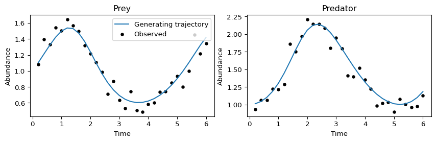
We observe both populations with independent Gaussian measurement noise of known standard deviation \(\sigma=0.1\). The dynamics themselves are deterministic. This additive noise is a simple measurement model for these synthetic abundance values; other measurements may require a different likelihood.

truth = {"alpha": 1.5, "gamma": 1.0}
sigma = 0.1
clean = predict(**truth)
observed = clean + sigma * jax.random.normal(jax.random.key(0), clean.shape)

fig, axes = plt.subplots(1, 2, figsize=(9, 3), sharex=True)
for i, (ax, name) in enumerate(zip(axes, ("Prey", "Predator"))):
    ax.plot(times, clean[:, i], label="Generating trajectory")
    ax.scatter(times, observed[:, i], s=15, color="black", label="Observed")
    ax.set(xlabel="Time", ylabel="Abundance", title=name)
axes[0].legend()
fig.tight_layout()
plt.show()

3. State the probabilistic model

A prior describes parameter uncertainty before using these observations. The likelihood describes how observations vary around a simulated trajectory. The posterior combines them. Writing the observed abundances as \(z\):

\[ p(\alpha,\gamma\mid z) \propto p(z\mid\alpha,\gamma)\,p(\alpha)\,p(\gamma). \]

We choose independent log-normal priors to keep the rates positive. Both have median 1 and standard deviation 0.3 on the log scale. These are moderately concentrated teaching priors that should be reconsidered for other models. The observation noise matches the data generation above.

def model(data=None):
    alpha = numpyro.sample("alpha", dist.LogNormal(0.0, 0.3))
    gamma = numpyro.sample("gamma", dist.LogNormal(0.0, 0.3))
    trajectory = predict(alpha, gamma)
    numpyro.deterministic("trajectory", trajectory)
    numpyro.sample("obs", dist.Normal(trajectory, sigma).to_event(2), obs=data)

numpyro.sample names the unknown parameters and records their densities. With obs=data, the last line scores the actual measurements. With data=None, it instead generates hypothetical observations. .to_event(2) sums the independent Normal log densities across times and populations; it does not add correlations.

There are no tvboptim Parameter wrappers here: NumPyro’s sample sites identify the unknowns and manage their positivity transformations.

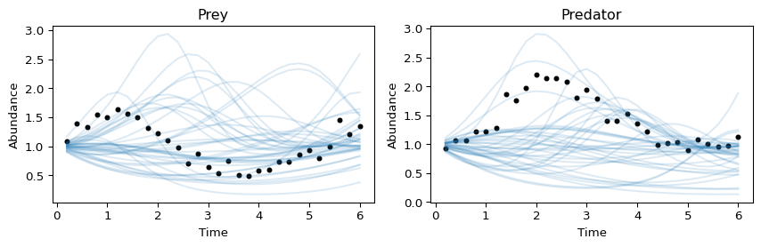
Before fitting, inspect noiseless trajectories from prior parameter draws. Their spread shows the response uncertainty before conditioning on the recording. For a real application, use scientific knowledge to assess whether these trajectories are plausible.

prior = Predictive(model, num_samples=40)(jax.random.key(1))

fig, axes = plt.subplots(1, 2, figsize=(9, 3))
for i, ax in enumerate(axes):
    ax.plot(times, prior["trajectory"][:, :, i].T, color="tab:blue", alpha=0.15)
    ax.scatter(times, observed[:, i], s=12, color="black")
    ax.set(xlabel="Time", ylabel="Abundance", title=("Prey", "Predator")[i])
fig.tight_layout()
plt.show()

4. Sample with Hamiltonian Monte Carlo (HMC)

HMC is a Markov chain Monte Carlo (MCMC) method. It uses gradients of the log posterior and auxiliary momentum to propose moves through parameter space. NUTS is an HMC variant that adapts the trajectory length. During warmup it also tunes sampling parameters; warmup draws are excluded from the reported posterior.

Each gradient evaluation differentiates through our ODE solve. NUTS targets the posterior defined by the priors, likelihood, and numerical solver, but a finite run can explore it poorly. Diagnostics are part of the inference.

mcmc = MCMC(
    NUTS(model),
    num_warmup=400,
    num_samples=600,
    num_chains=2,
    chain_method="sequential",
    progress_bar=False,
)
mcmc.run(jax.random.key(2), data=observed)
mcmc.print_summary(exclude_deterministic=True)
print("Divergences:", int(mcmc.get_extra_fields()["diverging"].sum()))
nuts_samples = {name: mcmc.get_samples()[name] for name in truth}

                mean       std    median      5.0%     95.0%     n_eff     r_hat
     alpha      1.51      0.01      1.51      1.48      1.53    893.82      1.00
     gamma      0.99      0.01      0.99      0.96      1.01    909.02      1.00

Number of divergences: 0
Divergences: 0

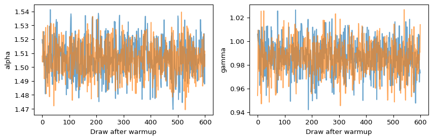
Check \(\hat R\) (R-hat), which compares variation within and between chains, effective sample size (ESS, reported as n_eff), and divergences. Look for R-hat at most 1.01, ESS of at least 200 for each inferred parameter, and no divergences; inspect chain traces as well. These are the screening thresholds used in the stimulation case study. The precision needed for a particular estimate, especially a tail probability, may require a larger ESS.

A divergence flags excessive numerical error along a Hamiltonian trajectory and can indicate that parts of the posterior are poorly explored. Investigate parameter scaling and model geometry; a higher target_accept_prob reduces the integration step size and may help. If ESS is low or R-hat is high, inspect chain mixing and initialization before extending the run. Also check the forward solver’s numerical accuracy. Passing these checks does not prove convergence or establish that disconnected posterior modes are absent.

chains = mcmc.get_samples(group_by_chain=True)
fig, axes = plt.subplots(1, 2, figsize=(9, 3))
for ax, name in zip(axes, truth):
    ax.plot(chains[name].T, alpha=0.65)
    ax.set(xlabel="Draw after warmup", ylabel=name)
fig.tight_layout()
plt.show()

5. Approximate the same posterior with SVI

SVI chooses a distribution \(q_\phi\), called a guide, and adjusts its parameters \(\phi\) to approximate the posterior. It maximizes the evidence lower bound (ELBO), trading off fit to the data against departure from the prior. Here the stochasticity comes from Monte Carlo estimates of the objective; we use all observations on every step.

AutoMultivariateNormal learns a Gaussian with correlations in the unconstrained coordinates (here, log rates). This makes fitting convenient, but cannot describe arbitrary posterior shapes or separated modes. See the NumPyro guide documentation.

guide = AutoMultivariateNormal(
    model,
    init_loc_fn=init_to_value(values={"alpha": 1.0, "gamma": 1.0}),
    init_scale=0.05,
)
svi = SVI(model, guide, Adam(0.005), Trace_ELBO(num_particles=8))
svi_result = svi.run(jax.random.key(3), 4000, data=observed, progress_bar=False)
svi_samples = guide.sample_posterior(
    jax.random.key(4), svi_result.params, sample_shape=(1200,),
)

fig, ax = plt.subplots(figsize=(6, 3))
ax.plot(svi_result.losses, alpha=0.6)
ax.set(xlabel="Optimization step", ylabel="Negative ELBO (lower is better)")
fig.tight_layout()
plt.show()

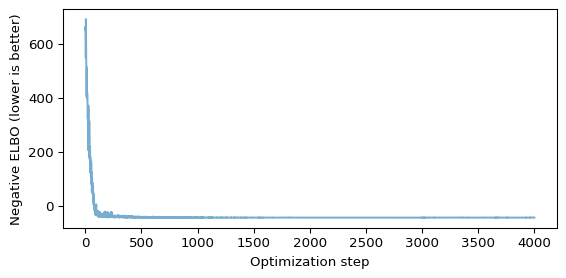
Both methods use the same model. Here SVI optimizes a distribution with a learned spread. Its speed and accuracy depend on the guide and optimization; a stable loss alone does not establish accurate uncertainty. Here we initialize at the prior medians, with a small spread in log rates, and average eight Monte Carlo draws per step to reduce noise in the objective. For your own problem, check sensitivity to initialization and optimization length.

6. Compare parameter uncertainty and predictions

A point estimate gives one parameter pair. Posterior draws also describe the remaining spread and dependence, conditional on the priors, observation model, and fixed quantities above.

Marginal distributions and credible intervals

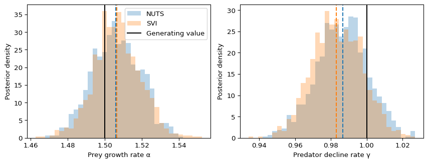
A marginal posterior describes one parameter while accounting for uncertainty in the other. The histograms below estimate these densities from NUTS and SVI draws. Their width shows remaining parameter uncertainty; their area is one. Dashed colored lines mark posterior medians, and the black line marks the known generating value.

parameter_samples = {"NUTS": nuts_samples, "SVI": svi_samples}
quantiles = jnp.array([0.05, 0.50, 0.95])
parameter_intervals = {
    label: {name: jnp.quantile(samples[name], quantiles) for name in truth}
    for label, samples in parameter_samples.items()
}

fig, axes = plt.subplots(1, 2, figsize=(9, 3.5))
for ax, name, title in zip(
    axes, truth, ("Prey growth rate α", "Predator decline rate γ")
):
    combined = jnp.concatenate([samples[name] for samples in parameter_samples.values()])
    bins = jnp.linspace(combined.min(), combined.max(), 36)
    for color, (label, samples) in zip(("tab:blue", "tab:orange"), parameter_samples.items()):
        ax.hist(samples[name], bins=bins, density=True, histtype="stepfilled",
                alpha=0.3, color=color, label=label)
        ax.axvline(float(parameter_intervals[label][name][1]), color=color, ls="--")
    ax.axvline(truth[name], color="black", label="Generating value")
    ax.set(xlabel=title, ylabel="Posterior density")
axes[0].legend()
fig.tight_layout()
plt.show()

For a compact numerical report, use the median and a 90% equal-tailed credible interval: the 5th and 95th percentiles, leaving 5% of the marginal posterior mass on either side. The table estimates these summaries from the draws; SVI intervals describe its fitted approximation.

from IPython.display import Markdown, display

rows = [
    "| Parameter | Method | Median | 90% credible interval | Generating value |",
    "|:--|:--|--:|:--|--:|",
]
for name in truth:
    for label in parameter_samples:
        lo, median, hi = parameter_intervals[label][name]
        rows.append(
            f"| {name} | {label} | {median:.3f} | [{lo:.3f}, {hi:.3f}] | {truth[name]:.3f} |"
        )
display(Markdown("\n".join(rows)))

Parameter	Method	Median	90% credible interval	Generating value
alpha	NUTS	1.506	[1.485, 1.526]	1.500
alpha	SVI	1.506	[1.486, 1.527]	1.500
gamma	NUTS	0.987	[0.962, 1.009]	1.000
gamma	SVI	0.983	[0.962, 1.007]	1.000

NUTS and SVI agree closely here. We infer only two rates, observe both populations, and keep the other quantities fixed. The narrow posterior appears approximately Gaussian in log-rate coordinates, which suits the guide. For skewed, curved, or multimodal posteriors, this guide may miss important structure. Agreement of medians and central intervals does not establish agreement in the tails or replace sampling diagnostics.

Under the specified model and given the observations, a 90% credible interval contains 90% of the parameter’s posterior probability. A frequentist confidence interval instead has a repeated-sampling coverage interpretation. We use “credible interval” for these Bayesian summaries.

The interval width describes uncertainty in the parameter, not numerical error in estimating its posterior median. More well-mixed NUTS draws improve Monte Carlo precision; they do not remove uncertainty caused by limited observations. A single synthetic fit also cannot establish that intervals are calibrated across repeated datasets.

Joint parameter uncertainty

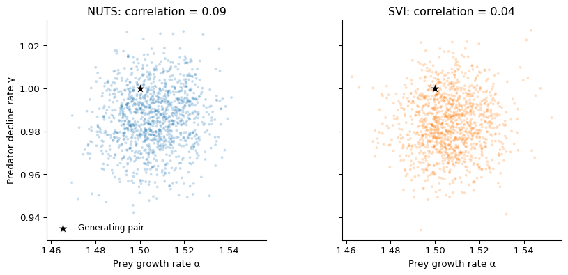
Marginal intervals do not show which parameter combinations are plausible together. Separate panels show the joint draws from each method on the same axes, with their sample correlation reported in the titles. In this example, dependence is weak, so the clouds can look nearly circular. A pronounced tilt is not a requirement for a valid posterior or a feature specific to NUTS: the SVI guide used here can also represent correlations. More NUTS draws improve the precision of the estimated correlation; they do not create stronger dependence. The stimulation case study provides a clearer parameter trade-off. The two marginal 90% intervals do not define a joint 90% credible region. The black star marks the generating parameter pair.

fig, axes = plt.subplots(1, 2, figsize=(9, 4), sharex=True, sharey=True,
                         layout="constrained")
for ax, (label, samples), color in zip(
    axes, parameter_samples.items(), ("tab:blue", "tab:orange")
):
    correlation = float(jnp.corrcoef(samples["alpha"], samples["gamma"])[0, 1])
    ax.scatter(samples["alpha"], samples["gamma"], s=8, alpha=0.25,
               color=color, edgecolors="none", rasterized=True)
    ax.scatter(truth["alpha"], truth["gamma"], color="black", marker="*", s=130,
               edgecolor="white", linewidth=0.6, label="Generating pair", zorder=5)
    ax.set(xlabel="Prey growth rate α", title=f"{label}: correlation = {correlation:.2f}")
    ax.set_box_aspect(1)
    ax.spines[["top", "right"]].set_visible(False)
axes[0].set_ylabel("Predator decline rate γ")
axes[0].legend(frameon=False, fontsize=9)
plt.show()

From parameter uncertainty to predictive intervals

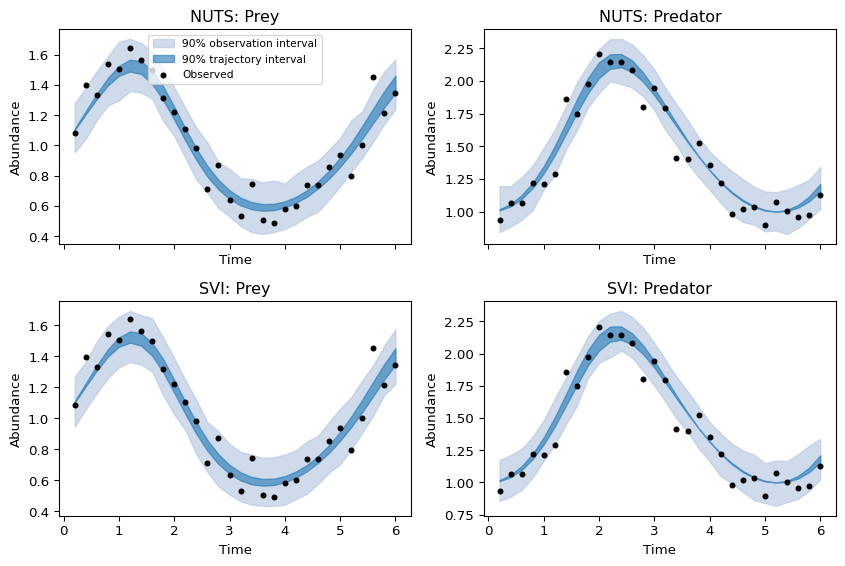
A posterior predictive check asks what new measurements the fitted model would produce. The trajectory interval reflects parameter uncertainty; the observation interval additionally includes measurement noise. We keep complete parameter pairs and use draws from both NUTS chains. The 90% intervals are pointwise at the recorded times, not simultaneous bands over the entire response. These checks reuse the fitting data; they do not validate predictions on a new recording.

posterior_predictions = {}
for seed, (label, samples) in enumerate(
    (("NUTS", nuts_samples), ("SVI", svi_samples)), start=5,
):
    # Evenly spaced draws span both sequential NUTS chains.
    take = jnp.linspace(0, len(samples["alpha"]) - 1, 300).astype(int)
    draws = {name: samples[name][take] for name in truth}
    posterior_predictions[label] = Predictive(model, posterior_samples=draws)(
        jax.random.key(seed)
    )

fig, axes = plt.subplots(2, 2, figsize=(9, 6), sharex=True)
for row, (label, predictions) in enumerate(posterior_predictions.items()):
    for i, ax in enumerate(axes[row]):
        for site, color, caption in (
            ("obs", "lightsteelblue", "90% observation interval"),
            ("trajectory", "tab:blue", "90% trajectory interval"),
        ):
            lo, hi = jnp.quantile(predictions[site][:, :, i], jnp.array([0.05, 0.95]), axis=0)
            ax.fill_between(times, lo, hi, color=color, alpha=0.6, label=caption)
        ax.scatter(times, observed[:, i], s=12, color="black", label="Observed")
        ax.set(title=f"{label}: {('Prey', 'Predator')[i]}", xlabel="Time", ylabel="Abundance")
axes[0, 0].legend(fontsize=8)
fig.tight_layout()
plt.show()

Using your own model

Replace predict with your prepared tvboptim simulation, align its outputs with your measurement times, and define priors and a likelihood appropriate to those measurements. The NUTS and SVI calls can retain the same structure.

Before interpreting an ODE posterior, check that reducing the integration step (or tightening adaptive solver tolerances) does not materially change predictions and inference. The posterior here is conditional on known initial conditions, fixed interaction rates, known noise, and the chosen observation model. Relaxing those assumptions can increase uncertainty and make inference harder.

For a next experiment, observe fewer time points and repeat both fits: how do the parameter cloud and predictive intervals change? Then try inferring the noise scale with a positive prior.

Continue with Bayesian Stimulation Inference: Identifiability and Prior Sensitivity to study an experiment where different parameter combinations produce similar responses. It connects Fisher information, posterior dependence, and shifted priors, then compares posterior draws with maximum a posteriori (MAP) point estimates. Both optimization and sampling can incorporate priors; the posterior distribution also describes the uncertainty around a point estimate.

Further directions

For larger models, inference cost depends on simulation and differentiation cost, posterior geometry, and the number of parameters. A dense NUTS mass matrix uses quadratic storage in parameter count; faster gradients alone do not make large inference problems easy. The NumPyro SVI guide extends the variational approach used here, but the guide family and convergence still need checking against diagnostics and, where feasible, posterior samples.

When a likelihood is difficult to evaluate, neural simulation-based inference (SBI) offers another route: draw parameters from a prior, simulate observations or summaries, and train a conditional density estimator to approximate the posterior. The sbi Bayesian workflow describes this process and its validation. Summary choice can discard information; training simulations and calibration checks are additional costs, and SBI does not automatically solve high-dimensional inference.

If the goal is to explore competing objectives, see the parallel Pareto optimization workflow. A Pareto front describes objective trade-offs; Bayesian uncertainty still requires a probabilistic model and inference.