---
title: "Stochastic Processes & Noise"
format:
html:
code-fold: false
toc: true
toc-depth: 3
fig-width: 8
out-width: "100%"
jupyter: python3
execute:
cache: true
---
Real neural systems exhibit intrinsic variability from multiple sources: spontaneous channel opening, synaptic fluctuations, and background activity. Stochastic processes capture this variability through noise terms in differential equations, transforming ODEs into stochastic differential equations (SDEs):
$$
\frac{d\mathbf{x}}{dt} = f(t, \mathbf{x}, \theta) + g(t, \mathbf{x}, \theta) \cdot \frac{d\mathbf{W}}{dt}
$$
where $f$ is the deterministic drift (dynamics), $g$ is the diffusion coefficient (noise intensity), and $d\mathbf{W}$ is Brownian motion.
The noise framework provides the diffusion coefficient $g(t, \mathbf{x}, \theta)$, while Diffrax SDE solvers handle the Brownian motion integration.
# The AbstractNoise Interface
All noise processes inherit from `AbstractNoise` and implement the diffusion coefficient:
```python
from tvboptim.experimental.network_dynamics.noise import AbstractNoise

class MyNoise(AbstractNoise):
    DEFAULT_PARAMS = Bunch(sigma=0.1)

    def diffusion(self, t: float, state: jnp.ndarray,
                  params: Bunch) -> jnp.ndarray:
        """Compute diffusion coefficient g(t, state, params).

        Args:
            t: Current time
            state: Current state [n_states, n_nodes]
            params: Noise parameters

        Returns:
            Diffusion coefficient [n_noise_states, n_nodes]
        """
        return params.sigma
```
Key features:
- **Selective application**: Use `apply_to` to add noise to specific states only
- `apply_to=None`: All states (default)
- `apply_to="V"`: Single state by name
- `apply_to=["V", "W"]`: Multiple states by name
- `apply_to=[0, 2]`: States by index
- **Parameter system**: Same pattern as dynamics and coupling (`DEFAULT_PARAMS`, can be overridden in constructor)
- **Integration**: Works with Diffrax SDE solvers and native solvers
# Additive Noise
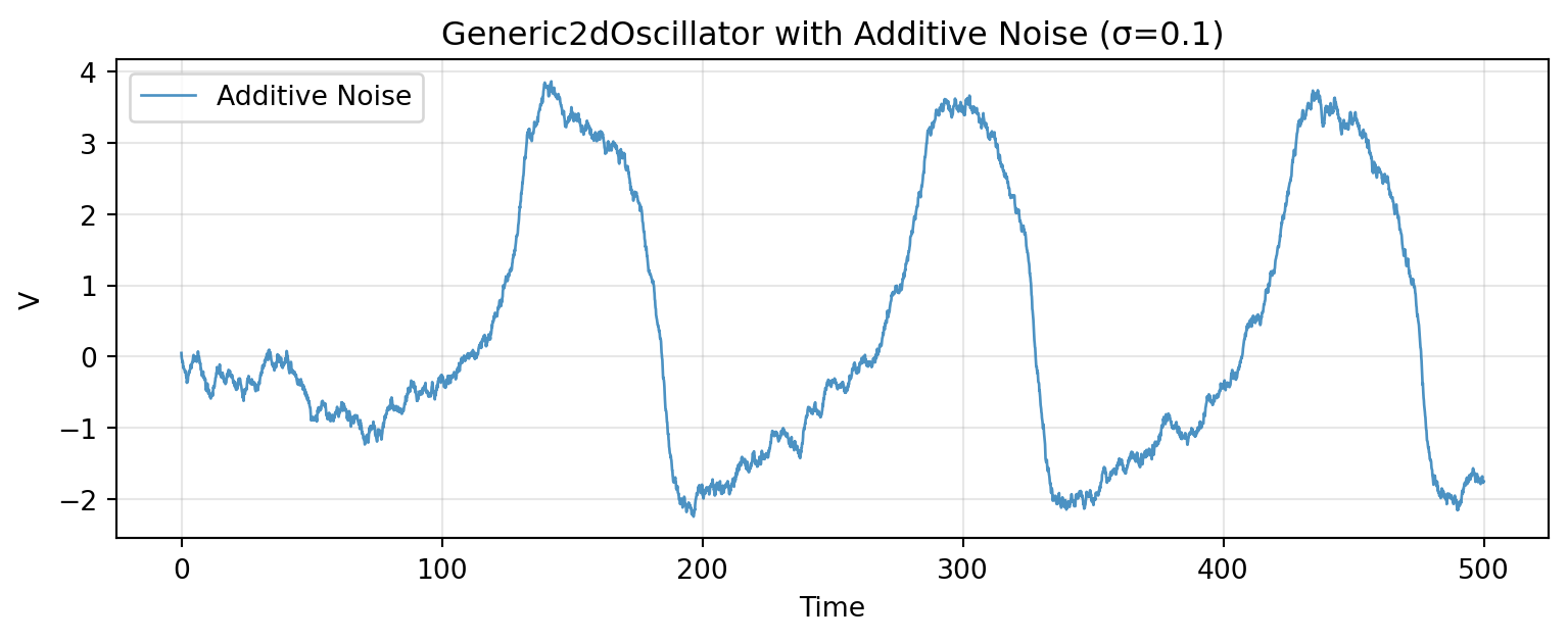
Additive noise has constant variance: $g(\mathbf{x}) = \sigma$.
```{python}
import jax
import jax.numpy as jnp
from tvboptim.experimental.network_dynamics import Network, solve
from tvboptim.experimental.network_dynamics.dynamics.tvb import Generic2dOscillator
from tvboptim.experimental.network_dynamics.noise import AdditiveNoise
from tvboptim.experimental.network_dynamics.coupling import LinearCoupling
from tvboptim.experimental.network_dynamics.graph import DenseGraph
from tvboptim.experimental.network_dynamics.solvers import Euler

# Create network with additive noise
dynamics = Generic2dOscillator()
noise = AdditiveNoise(sigma=0.1)
coupling = LinearCoupling(incoming_states="V", G=0.5)
graph = DenseGraph.random(n_nodes=10, sparsity=0.3, key=jax.random.key(0))

network_additive = Network(dynamics=dynamics, coupling={'instant': coupling},
                           graph=graph, noise=noise)

# Simulate with Euler solver (handles noise automatically)
result_additive = solve(network_additive, Euler(),
                        t0=0.0, t1=500.0, dt=0.1)

print(f"Result shape: {result_additive.ys.shape}")  # [time, states, nodes]
```
```{python}
#| code-fold: true
#| code-summary: "Visualization"
import matplotlib.pyplot as plt

fig, ax = plt.subplots(figsize=(8.1, 3.375))

# Plot V trajectory
t = result_additive.ts
V_additive = result_additive.ys[:, 0, 0]  # First state, first node

ax.plot(t, V_additive, linewidth=1, alpha=0.8, label='Additive Noise')
ax.set_xlabel('Time')
ax.set_ylabel('V')
ax.set_title('Generic2dOscillator with Additive Noise (σ=0.1)')
ax.legend()
ax.grid(True, alpha=0.3)

plt.tight_layout()
plt.show()
```
The noise intensity remains constant regardless of the oscillation amplitude.
# Multiplicative Noise
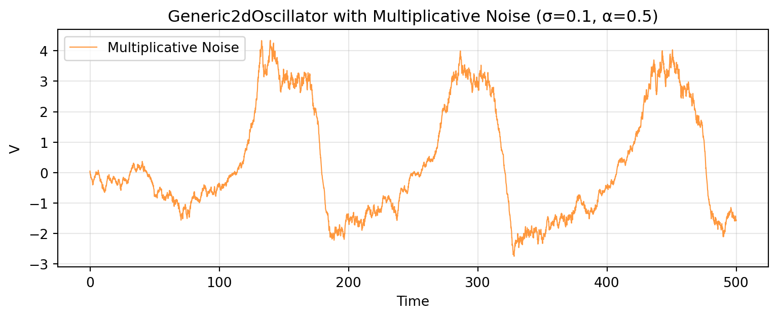
Multiplicative noise scales with state magnitude: $g(\mathbf{x}) = \sigma \cdot (1 + \alpha |\mathbf{x}|)$.
To demonstrate how to implement custom noise, let's create our own multiplicative noise class:
```{python}
from tvboptim.experimental.network_dynamics.noise import AbstractNoise
from tvboptim.experimental.network_dynamics.core.bunch import Bunch

class MyMultiplicativeNoise(AbstractNoise):
    """Custom multiplicative noise implementation.

    Noise intensity increases with state magnitude, creating
    state-dependent fluctuations.
    """

    DEFAULT_PARAMS = Bunch(
        sigma=0.1,           # Base noise level
        state_scaling=0.5    # How strongly noise scales with state
    )

    def diffusion(self, t: float, state: jnp.ndarray,
                  params: Bunch) -> jnp.ndarray:
        """Compute state-dependent diffusion coefficient.

        Returns: sigma * (1 + alpha * |state|)
        """
        # Extract states that receive noise (determined by apply_to)
        relevant_states = state[self._state_indices]

        # Scale noise by state magnitude
        scaling = 1.0 + params.state_scaling * jnp.abs(relevant_states)
        return params.sigma * scaling
```
Now use our custom noise class:
```{python}
# Same network structure, custom multiplicative noise
noise_mult = MyMultiplicativeNoise(sigma=0.1, state_scaling=0.5)

network_mult = Network(dynamics=dynamics, coupling={'instant': coupling},
                       graph=graph, noise=noise_mult)

result_mult = solve(network_mult, Euler(),
                    t0=0.0, t1=500.0, dt=0.1)
```
```{python}
#| code-fold: true
#| code-summary: "Visualization"
fig, ax = plt.subplots(figsize=(8.1, 3.375))

V_mult = result_mult.ys[:, 0, 0]

ax.plot(t, V_mult, linewidth=0.8, alpha=0.8, label='Multiplicative Noise', color='C1')
ax.set_xlabel('Time')
ax.set_ylabel('V')
ax.set_title('Generic2dOscillator with Multiplicative Noise (σ=0.1, α=0.5)')
ax.legend()
ax.grid(True, alpha=0.3)

plt.tight_layout()
plt.show()
```
The noise intensity increases during large amplitude excursions, creating state-dependent variability.
# Comparison: Additive vs Multiplicative
```{python}
#| code-fold: true
#| code-summary: "Visualization"
fig, ax = plt.subplots(figsize=(8.1, 3.375))
# Plot both traces in same panel for direct comparison
ax.plot(t, V_additive, linewidth=0.8, alpha=0.7, label='Additive (constant σ)')
ax.plot(t, V_mult, linewidth=0.8, alpha=0.7, label='Multiplicative (state-dependent)')
ax.set_xlabel('Time')
ax.set_ylabel('V')
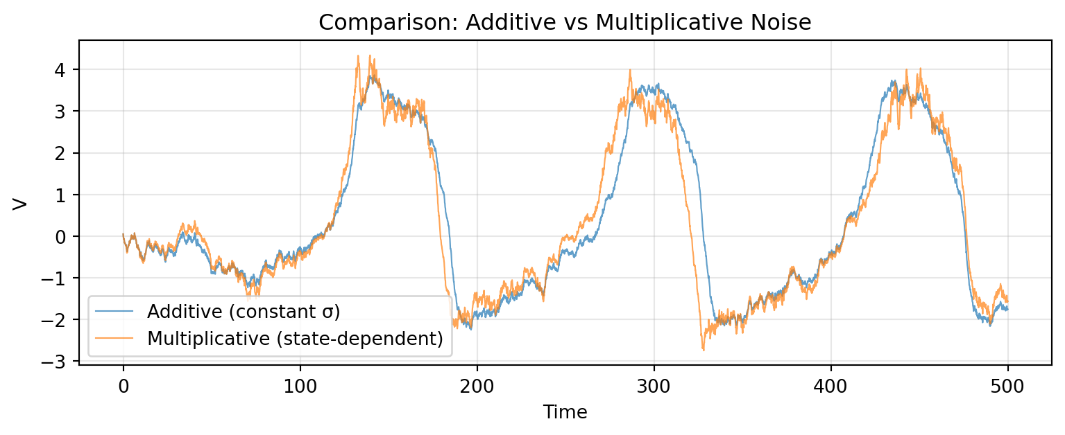
ax.set_title('Comparison: Additive vs Multiplicative Noise')
ax.legend()
ax.grid(True, alpha=0.3)
plt.tight_layout()
plt.show()
```
Multiplicative noise amplifies fluctuations during large oscillations, while additive noise maintains constant variance throughout.
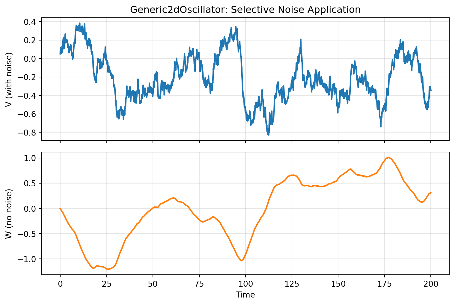
# Selective Noise Application
The `apply_to` parameter restricts noise to specific state variables:
```{python}
# Generic2dOscillator with noise only on first state (V), not second (W)
dynamics_selective = Generic2dOscillator()
noise_selective = AdditiveNoise(sigma=0.1, apply_to="V")
graph_single = DenseGraph(jnp.ones((1, 1)))  # Single node

network_selective = Network(dynamics=dynamics_selective, graph=graph_single,
                            noise=noise_selective, coupling={'instant': coupling})

# Verify configuration
noise_selective.verify(dynamics_selective)
```
```{python}
# Simulate
result_selective = solve(network_selective, Euler(),
                         t0=0.0, t1=200.0, dt=0.1)
```
```{python}
#| code-fold: true
#| code-summary: "Visualization"
fig, (ax1, ax2) = plt.subplots(2, 1, figsize=(8.1, 5.4), sharex=True)

t_sel = result_selective.ts
V_sel = result_selective.ys[:, 0, 0]  # V state
W_sel = result_selective.ys[:, 1, 0]  # W state

ax1.plot(t_sel, V_sel, linewidth=1.8)
ax1.set_ylabel('V (with noise)')
ax1.set_title('Generic2dOscillator: Selective Noise Application')
ax1.grid(True, alpha=0.3)

ax2.plot(t_sel, W_sel, linewidth=1.8, color='C1')
ax2.set_xlabel('Time')
ax2.set_ylabel('W (no noise)')
ax2.grid(True, alpha=0.3)

plt.tight_layout()
plt.show()
```
Only the first state variable V exhibits stochastic fluctuations, while the second variable W evolves deterministically.
# Summary
The noise framework enables stochastic simulations of network dynamics:
- **AbstractNoise interface**: Implement `diffusion(t, state, params)` to define noise intensity
- **Additive noise**: Constant variance, simplest model of background fluctuations
- **Multiplicative noise**: State-dependent variance, captures amplitude-dependent variability
- **Selective application**: Target specific state variables with `apply_to` parameter
- **Integration**: Works with both native solvers (Euler automatically handles noise) and Diffrax SDE solvers
The diffusion coefficient determines how noise enters the system, enabling realistic models of intrinsic neural variability.