---
title: "External Inputs in Network Dynamics"
format:
html:
code-fold: false
toc: true
toc-depth: 3
fig-width: 8
out-width: "100%"
jupyter: python3
execute:
cache: true
---
# Introduction
External inputs provide a flexible system for driving network dynamics with time-dependent (and optionally state-dependent) signals. Unlike coupling, which represents interactions between nodes, external inputs represent stimuli from outside the network - such as sensory input, experimental perturbations, or recorded data.
The external input system is designed to mirror the coupling architecture, using named dictionaries for routing inputs to the correct model variables.
## Key Features
- **Parametric Inputs**: Time-dependent functions with optimizable parameters
- **Data-based Inputs**: Interpolated time-series data that works with any simulation `dt`
- **Flexible Broadcasting**: Scalar parameters broadcast to all nodes, or specify per-node values
- **State-dependent Inputs**: Inputs can access network state for closed-loop stimulation
- **Named Routing**: Dictionary-based routing matches inputs to model variables (similar to coupling)
# Example 1: Creating a Custom Parametric Input
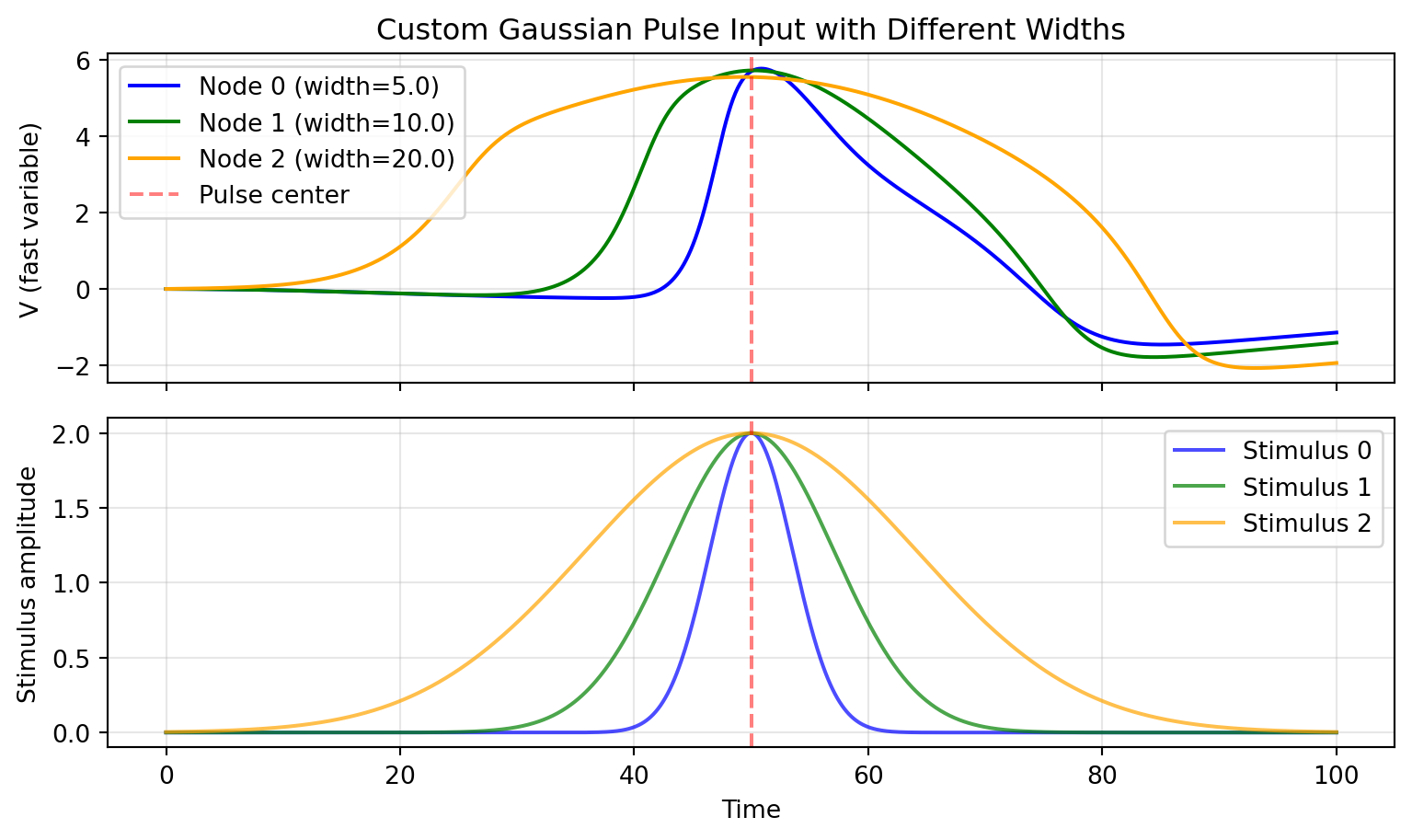
Let's learn how to create custom external inputs by implementing a Gaussian pulse - a smooth, bell-shaped stimulus useful for modeling transient perturbations.
## Defining the Custom Input Class
```{python}
import jax.numpy as jnp
from tvboptim.experimental.network_dynamics.core.bunch import Bunch
from tvboptim.experimental.network_dynamics.external_input import AbstractExternalInput

class GaussianPulseInput(AbstractExternalInput):
    """Gaussian pulse stimulus centered at a specific time.

    Creates a smooth bell-shaped pulse defined by:
        amplitude * exp(-((t - center) / width)^2)
    """

    N_OUTPUT_DIMS = 1  # Output is 1-dimensional

    DEFAULT_PARAMS = Bunch(
        center=50.0,      # Time of pulse peak
        width=10.0,       # Pulse width (standard deviation)
        amplitude=1.0,    # Pulse height
    )

    def prepare(self, network, dt):
        """Prepare for simulation (stateless, so nothing to do)."""
        return Bunch(), Bunch()  # (input_data, input_state)

    def compute(self, t, state, input_data, input_state, params):
        """Compute Gaussian pulse value at time t."""
        # Calculate Gaussian
        pulse = params.amplitude * jnp.exp(-((t - params.center) / params.width) ** 2)

        # Handle broadcasting: scalar → [1, n_nodes]
        if jnp.ndim(pulse) == 0:
            return jnp.full((1, state.shape[1]), pulse)
        else:
            return pulse[None, :]

    def update_state(self, input_data, input_state, new_state):
        """Update state (stateless, so return unchanged)."""
        return input_state

print("Custom GaussianPulseInput class defined!")
```
## Using the Custom Input
Now let's use our custom input to stimulate a network:
```{python}
from tvboptim.experimental.network_dynamics import Network, solve
from tvboptim.experimental.network_dynamics.dynamics.tvb import Generic2dOscillator
from tvboptim.experimental.network_dynamics.coupling import LinearCoupling
from tvboptim.experimental.network_dynamics.graph import DenseGraph
from tvboptim.experimental.network_dynamics.solvers import Euler

# Create excitable dynamics
dynamics = Generic2dOscillator(
    a=-2.0, b=-10.0, c=0.0, d=0.02,
    tau=1.0, I=0.0
)

# 3 nodes with different pulse widths
graph = DenseGraph(jnp.eye(3))
coupling = LinearCoupling(incoming_states='V', G=0.0)

# Create Gaussian pulse with per-node widths
gaussian_input = GaussianPulseInput(
    center=50.0,
    width=jnp.array([5.0, 10.0, 20.0]),  # Different widths per node
    amplitude=2.0
)

network = Network(
    dynamics=dynamics,
    coupling={'instant': coupling},
    graph=graph,
    external_input={'stimulus': gaussian_input}
)

print(network)
```
## Simulating and Visualizing
```{python}
import matplotlib.pyplot as plt

result = solve(network, Euler(), t0=0.0, t1=100.0, dt=0.1)

# Plot results
fig, (ax1, ax2) = plt.subplots(2, 1, figsize=(8.1, 4.86), sharex=True)

colors = ['blue', 'green', 'orange']
widths = [5.0, 10.0, 20.0]

for i in range(3):
    ax1.plot(result.ts, result.ys[:, 0, i],
             label=f'Node {i} (width={widths[i]})', color=colors[i])
ax1.axvline(50, color='red', linestyle='--', alpha=0.5, label='Pulse center')
ax1.set_ylabel('V (fast variable)')
ax1.legend()
ax1.grid(True, alpha=0.3)
ax1.set_title('Custom Gaussian Pulse Input with Different Widths')

# Plot the actual stimulus for reference using the built-in plot helper
gaussian_input.plot(0.0, 100.0, n_nodes=3, ax=ax2)
ax2.axvline(50, color='red', linestyle='--', alpha=0.5)
ax2.set_title('')
ax2.set_ylabel('Stimulus amplitude')
ax2.set_xlabel('Time')
ax2.legend([f'Stimulus {i}' for i in range(3)])
ax2.grid(True, alpha=0.3)

plt.tight_layout()
plt.show()
```
## Key Observations
- Narrower pulses (width=5) trigger sharp, localized responses
- Wider pulses (width=20) produce more sustained activation
- All three nodes receive pulses centered at t=50, but with different temporal profiles
- Parameters can be easily marked for optimization using `Parameter` types
# Example 2: Data-based Input with Interpolation
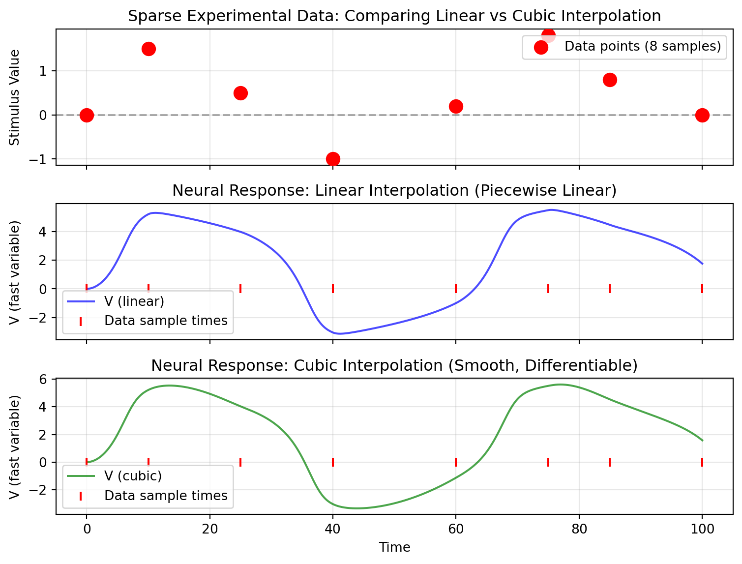
Data-based inputs are essential when you have recorded experimental data or want to precisely control the temporal structure of stimulation using pre-computed signals.
## Creating and Interpolating Sparse Data
```{python}
from tvboptim.experimental.network_dynamics.external_input import DataInput

# Simulate sparse experimental data (e.g., from recordings)
# Only 8 data points over 100 time units - very sparse!
data_times = jnp.array([0., 10., 25., 40., 60., 75., 85., 100.])
data_data = jnp.array([0., 1.5, 0.5, -1.0, 0.2, 1.8, 0.8, 0.])

print(f"Data points: {len(data_times)} samples over [0, 100]")
print(f"Average sampling interval: {jnp.mean(jnp.diff(data_times)):.1f}")
```
## Comparing Interpolation Methods
```{python}
# Create two inputs with different interpolation methods
linear_stimulus = DataInput(data_times, data_data, interpolation='linear')
cubic_stimulus = DataInput(data_times, data_data, interpolation='cubic')

# Build networks
network_linear = Network(
    dynamics=dynamics,
    coupling={'instant': coupling},
    graph=DenseGraph(jnp.eye(1)),  # Single node
    external_input={'stimulus': linear_stimulus}
)

network_cubic = Network(
    dynamics=dynamics,
    coupling={'instant': coupling},
    graph=DenseGraph(jnp.eye(1)),
    external_input={'stimulus': cubic_stimulus}
)

# Simulate with fine dt (10x finer than average data sampling)
dt_sim = 0.1
print(f"\nSimulation dt: {dt_sim} (much finer than data sampling)")

result_linear = solve(network_linear, Euler(), t0=0.0, t1=100.0, dt=dt_sim)
result_cubic = solve(network_cubic, Euler(), t0=0.0, t1=100.0, dt=dt_sim)
```
## Visualizing Interpolation Quality
```{python}
fig, (ax1, ax2, ax3) = plt.subplots(3, 1, figsize=(8.1, 6.075), sharex=True)

# Plot 1: Show original sparse data points alongside the two interpolated stimuli
linear_stimulus.plot(0.0, 100.0, ax=ax1)
cubic_stimulus.plot(0.0, 100.0, ax=ax1)
ax1.scatter(data_times, data_data, s=100, c='red', zorder=5, label='Data points (8 samples)')
ax1.axhline(0, color='k', linestyle='--', alpha=0.3)
ax1.set_ylabel('Stimulus Value')
ax1.legend(['linear', 'cubic', 'Data points (8 samples)'])
ax1.grid(True, alpha=0.3)
ax1.set_title('Sparse Experimental Data: Comparing Linear vs Cubic Interpolation')

# Plot 2: Neural response with linear interpolation
ax2.plot(result_linear.ts, result_linear.ys[:, 0, 0], 'b-', label='V (linear)', alpha=0.7)
ax2.scatter(data_times, jnp.zeros_like(data_times), s=50, c='red',
            marker='|', zorder=5, label='Data sample times')
ax2.set_ylabel('V (fast variable)')
ax2.legend()
ax2.grid(True, alpha=0.3)
ax2.set_title('Neural Response: Linear Interpolation (Piecewise Linear)')

# Plot 3: Neural response with cubic interpolation
ax3.plot(result_cubic.ts, result_cubic.ys[:, 0, 0], 'g-', label='V (cubic)', alpha=0.7)
ax3.scatter(data_times, jnp.zeros_like(data_times), s=50, c='red',
            marker='|', zorder=5, label='Data sample times')
ax3.set_ylabel('V (fast variable)')
ax3.set_xlabel('Time')
ax3.legend()
ax3.grid(True, alpha=0.3)
ax3.set_title('Neural Response: Cubic Interpolation (Smooth, Differentiable)')

plt.tight_layout()
plt.show()
```
The cubic interpolation produces smoother dynamics between data points, which is often more realistic for biological signals.
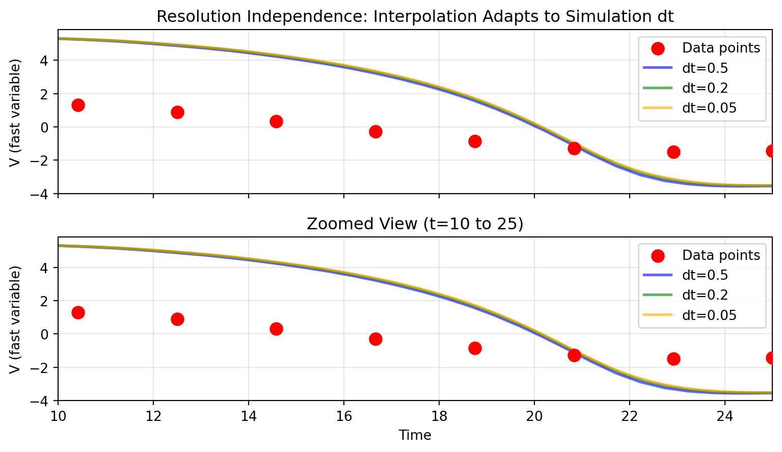
## Resolution Independence
A key advantage of interpolation-based inputs: the same data works seamlessly with any simulation `dt`:
```{python}
# Use moderate data sampling
data_times = jnp.linspace(0, 50, 25)  # 25 points, dt ≈ 2.08
data_data = jnp.sin(data_times * 0.2) * 1.5

data_stimulus = DataInput(data_times, data_data, interpolation='cubic')

# Test with three different simulation dt values
dt_values = [0.5, 0.2, 0.05]
results = []

print("Same data, different simulation resolutions:")
for dt in dt_values:
    network = Network(
        dynamics=dynamics,
        coupling={'instant': coupling},
        graph=DenseGraph(jnp.eye(1)),
        external_input={'stimulus': data_stimulus}
    )
    result = solve(network, Euler(), t0=0.0, t1=50.0, dt=dt)
    results.append(result)
    print(f"  dt={dt:4.2f}: {len(result.ts):4d} time steps")
```
```{python}
# Visualize resolution independence
fig, (ax1, ax2) = plt.subplots(2, 1, figsize=(8.1, 4.725), sharex=True)

# Full time range
ax1.scatter(data_times, data_data, s=80, c='red', zorder=5, label='Data points')
colors = ['blue', 'green', 'orange']
for dt, result, color in zip(dt_values, results, colors):
    ax1.plot(result.ts, result.ys[:, 0, 0], alpha=0.6,
             label=f'dt={dt}', linewidth=2, color=color)
ax1.set_ylabel('V (fast variable)')
ax1.legend()
ax1.grid(True, alpha=0.3)
ax1.set_title('Resolution Independence: Interpolation Adapts to Simulation dt')

# Zoomed view to see detail
ax2.scatter(data_times, data_data, s=80, c='red', zorder=5, label='Data points')
for dt, result, color in zip(dt_values, results, colors):
    ax2.plot(result.ts, result.ys[:, 0, 0], alpha=0.6,
             label=f'dt={dt}', linewidth=2, color=color)
ax2.set_xlim(10, 25)
ax2.set_ylabel('V (fast variable)')
ax2.set_xlabel('Time')
ax2.legend()
ax2.grid(True, alpha=0.3)
ax2.set_title('Zoomed View (t=10 to 25)')

plt.tight_layout()
plt.show()
```
All three simulations produce consistent results because Diffrax interpolation evaluates the stimulus at whatever time points the solver requests.
# Integration with Models
## Declaring External Inputs in Dynamics
Models declare which external inputs they accept via the `EXTERNAL_INPUTS` class attribute:
```{python}
#| eval: false
# Example from Generic2dOscillator
class Generic2dOscillator(AbstractDynamics):
    EXTERNAL_INPUTS = {'stimulus': 1}  # Accepts 1D 'stimulus' input

    def dynamics(self, t, state, params, coupling, external):
        # Access external input by name
        stim = external.stimulus[0]  # Extract [1, n_nodes] -> [n_nodes]

        # Use in dynamics equations
        dV = ... + stim
        return jnp.stack([dV, dW])
```
The key `'stimulus'` matches the name used when creating the network, and the value `1` indicates it's 1-dimensional.
## Network Creation with Named Routing
```{python}
#| eval: false
network = Network(
    dynamics=dynamics,
    coupling={'instant': coupling_instant},
    graph=graph,
    external_input={'stimulus': gaussian_input}  # Name must match EXTERNAL_INPUTS
)
```
The external input system automatically:
1. Validates input names match `EXTERNAL_INPUTS` declarations
2. Prepares interpolators (for `DataInput`)
3. Handles broadcasting based on parameter shapes
4. Pre-compiles computations for performance
# Tips and Best Practices
## When to Use Which Input Type
**Parametric Inputs** (like `SineInput`, or custom `GaussianPulseInput`):
- When you want to optimize stimulus parameters
- For idealized, controlled stimulation protocols
- When stimulus is defined by a mathematical function
**Data-based Inputs** (`DataInput`):
- When you have experimental recordings
- For complex temporal patterns that are hard to parameterize
- When you need to replay specific stimulus sequences
## Choosing Interpolation
- **Linear**: Fast, simple, good for densely sampled data (>10 samples per characteristic timescale)
- **Cubic**: Smooth and differentiable, better for sparse data or when derivatives matter
## Parameter Optimization
External input parameters integrate with the parameter system:
```{python}
#| eval: false
from tvboptim.types import Parameter, BoundedParameter

# Mark parameters for optimization
gaussian_input = GaussianPulseInput(
    center=Parameter(50.0),                          # Optimize pulse timing
    width=BoundedParameter(10.0, low=1.0, high=50.0), # Constrained width
    amplitude=2.0                                     # Fixed amplitude
)
```
## Performance Considerations
- Parametric inputs are evaluated at each time step (fast, simple functions)
- Data interpolation (especially cubic) adds computation but is still JIT-compiled
- For very long simulations with data inputs, consider your data sampling rate
# Summary
The external input system provides:
- **Extensibility**: Easy to create custom inputs by subclassing `AbstractExternalInput`
- **Flexibility**: Both parametric and data-based inputs work seamlessly
- **Integration**: Named routing matches coupling system architecture
- **Performance**: JIT-compiled for efficiency in long simulations
For complete examples with multiple input types and network configurations, see:
- `examples/external_input_demo.py`: Parametric inputs (sine, pulse, etc.)
- `examples/data_input_demo.py`: Data interpolation and per-node stimulation