---
title: "Coupling"
format:
html:
code-fold: false
toc: true
toc-depth: 3
fig-width: 8
out-width: "100%"
jupyter: python3
execute:
cache: true
---
# Introduction
Coupling defines how network nodes interact through structural connectivity. While dynamics govern local temporal evolution at each node, coupling transmits information between nodes, enabling collective behaviors like synchronization, wave propagation, and functional integration.
The general form of coupling input is:
$$
c_i = \sum_{j} w_{ij} \cdot f(\text{state}_j, \text{state}_i, \theta)
$$
where $w_{ij}$ represents connection weights from the graph, and $f$ is the coupling function with parameters $\theta$.
# Coupling in Network Dynamics
Coupling integrates with dynamics through named input channels. The `dynamics()` method receives coupling as a `Bunch` object with named attributes:
```python
def dynamics(self, t, state, params, coupling, external):
    # Access coupling inputs by name
    c_instant = coupling.instant[0]
    c_delayed = coupling.delayed[0]

    # Use in dynamics equations
    dX_dt = ... + c_instant + c_delayed
    return derivatives
```
Networks support multiple coupling types through a named dictionary:
```{python}
import jax.numpy as jnp
from tvboptim.experimental.network_dynamics import Network, solve
from tvboptim.experimental.network_dynamics.dynamics import ReducedWongWang
from tvboptim.experimental.network_dynamics.coupling import LinearCoupling
from tvboptim.experimental.network_dynamics.graph import DenseGraph
from tvboptim.experimental.network_dynamics.solvers import Euler

# Create simple network
dynamics = ReducedWongWang()
graph = DenseGraph(jnp.array([[0.0, 1.0], [1.0, 0.0]]))
coupling = LinearCoupling(incoming_states='S', G=0.5)

network = Network(
    dynamics=dynamics,
    coupling={'instant': coupling},  # Named coupling
    graph=graph
)

print(network)
```
**Key point**: If a dynamics model declares coupling inputs that are not provided in the network, those inputs are automatically filled with zeros. This allows flexible network configurations without requiring all possible couplings.
# The Coupling API
Coupling objects follow a three-phase lifecycle that mirrors the simulation flow:
## Phase 1: Preparation (*prepare*)
Called once before simulation starts:
```python
coupling_data, coupling_state = coupling.prepare(network, dt)
```
**Returns**:
- `coupling_data` (Bunch): Static precomputed data
- State indices to extract from network state
- Delay step indices (for delayed coupling)
- Optimization flags (sparse/dense modes)
- `coupling_state` (Bunch): Mutable internal state
- History buffers (for delayed coupling)
- Empty for instantaneous coupling
## Phase 2: Computation (*compute*)
Called every time step during integration:
```python
coupling_input = coupling.compute(t, state, coupling_data,
                                   coupling_state, params, graph)
```
**Returns**:
- Coupling input array `[n_coupling_dims, n_nodes]`
## Phase 3: State Update (*update_state*)
Called after each integration step:
```python
coupling_state = coupling.update_state(coupling_data,
                                       coupling_state, new_state)
```
**Returns**:
- Updated `coupling_state` (e.g., updated history buffer)
**Flow pseudocode**:
```python
# Before simulation
coupling_data, coupling_state = coupling.prepare(network, dt)

# During simulation (at each time step)
for step in range(n_steps):
    # Compute coupling input
    coupling_input = coupling.compute(t, state, coupling_data,
                                      coupling_state, params, graph)

    # Integrate dynamics (uses coupling_input)
    new_state = integrate_step(state, coupling_input, dt)

    # Update coupling state
    coupling_state = coupling.update_state(coupling_data,
                                           coupling_state, new_state)
    state = new_state
```
# TVB-Style Couplings: Pre and Post Pattern
Most brain network models follow a standard coupling pattern: transform states before aggregation (`pre`), perform weighted summation, then transform the result (`post`). This pattern is captured in the `InstantaneousCoupling` and `DelayedCoupling` base classes.
The computation flow is:
```
pre(states) → weighted sum → post(sum)
```
## LinearCoupling Example
The simplest coupling applies a gain and offset to the weighted sum:
```{python}
from tvboptim.experimental.network_dynamics.coupling import LinearCoupling

# Create linear coupling
coupling = LinearCoupling(incoming_states='x', G=2.0, b=0.1)

print(f"Coupling parameters: G={coupling.params.G}, b={coupling.params.b}")
print(f"Incoming states: {coupling.INCOMING_STATE_NAMES}")
```
The `post()` implementation is simple:
```python
def post(self, summed_inputs, local_states, params):
    return params.G * summed_inputs + params.b
```
Since `pre()` is not overridden, it returns incoming states unchanged (identity function).
## DifferenceCoupling: Overriding Pre
When coupling depends on differences between nodes, we override `pre()`:
```{python}
from tvboptim.experimental.network_dynamics.coupling import DifferenceCoupling

# Difference coupling: couples based on (x_j - x_i)
diff_coupling = DifferenceCoupling(
    incoming_states='x',
    local_states='x',  # Need local state for difference
    G=1.0
)

print(f"Incoming states: {diff_coupling.INCOMING_STATE_NAMES}")
print(f"Local states: {diff_coupling.LOCAL_STATE_NAMES}")
```
The `pre()` method computes differences:
```python
def pre(self, incoming_states, local_states, params):
    # incoming_states: [n_states, n_nodes, n_nodes] per-edge format
    # local_states: [n_states, n_nodes]
    return incoming_states - local_states[:, :, None]
```
This enables synchronization dynamics where coupling strength depends on state mismatch.
# Vectorized vs Per-Edge Modes
A key performance consideration is how coupling interacts with the connectivity matrix. TVB-Optim supports two modes:
**Per-Edge Mode (3D)**: `pre()` returns `[n_states, n_nodes, n_nodes]`
- Element-wise multiply with weights: `pre_states * weights`
- Then sum over source nodes
- Flexible: supports per-connection transformations
- Slower for dense graphs
**Vectorized Mode (2D)**: `pre()` returns `[n_states, n_nodes]`
- Matrix multiplication: `pre_states @ weights`
- Faster for dense graphs (optimized BLAS)
- Less flexible: same operation for all connections
## LinearCoupling vs FastLinearCoupling
`FastLinearCoupling` achieves vectorized mode by using `local_states` instead of `incoming_states`:
```{python}
from tvboptim.experimental.network_dynamics.coupling import FastLinearCoupling

# Standard: uses incoming_states (per-edge)
standard = LinearCoupling(incoming_states='S', G=1.0)

# Fast: uses local_states (vectorized)
fast = FastLinearCoupling(local_states='S', G=1.0)

print("Standard coupling mode: per-edge (3D)")
print("Fast coupling mode: vectorized (2D)")
```
The difference is in `pre()`:
```python
# LinearCoupling: inherits default pre() returning incoming_states (3D)
# → per-edge mode

# FastLinearCoupling:
def pre(self, incoming_states, local_states, params):
    return local_states  # 2D → vectorized mode
```
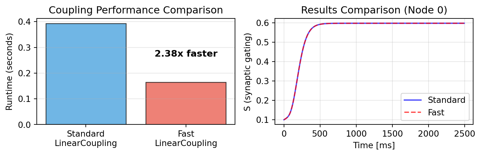
## Performance Benchmark
Let's compare runtime with empirical connectivity (84 regions, 5000 time steps):
```{python}
import time
from tvboptim.data import load_structural_connectivity
from tvboptim.experimental.network_dynamics.dynamics.tvb import ReducedWongWang
from tvboptim.experimental.network_dynamics.solvers import Heun

# Load empirical connectivity
weights, lengths, labels = load_structural_connectivity("dk_average")
weights_norm = weights / jnp.max(weights)  # Normalize

print(f"Network size: {weights.shape[0]} nodes")
print(f"Simulation: 5000 steps (dt=0.5 ms)")

# Setup
dynamics = ReducedWongWang()
graph = DenseGraph(weights_norm)

# Standard LinearCoupling (per-edge mode)
coupling_standard = LinearCoupling(incoming_states='S', G=0.5)
network_standard = Network(dynamics=dynamics, coupling={'instant': coupling_standard}, graph=graph)

# FastLinearCoupling (vectorized mode)
coupling_fast = FastLinearCoupling(local_states='S', G=0.5)
network_fast = Network(dynamics=dynamics, coupling={'instant': coupling_fast}, graph=graph)

solver = Heun()
n_steps = 5000
dt = 0.5

# Benchmark: Standard coupling
start = time.time()
result_standard = solve(network_standard, solver, t0=0.0, t1=n_steps*dt, dt=dt)
time_standard = time.time() - start

# Benchmark: Fast coupling
start = time.time()
result_fast = solve(network_fast, solver, t0=0.0, t1=n_steps*dt, dt=dt)
time_fast = time.time() - start

print(f"\nStandard LinearCoupling: {time_standard:.3f} s")
print(f"FastLinearCoupling: {time_fast:.3f} s")
print(f"Speedup: {time_standard/time_fast:.2f}x")
```
```{python}
#| code-fold: true
#| code-summary: "Visualization"
import matplotlib.pyplot as plt

fig, (ax1, ax2) = plt.subplots(1, 2, figsize=(8.1, 2.7))

# Bar chart
couplings = ['Standard\nLinearCoupling', 'Fast\nLinearCoupling']
times = [time_standard, time_fast]
colors = ['#3498db', '#e74c3c']

ax1.bar(couplings, times, color=colors, alpha=0.7, edgecolor='black')
ax1.set_ylabel('Runtime (seconds)')
ax1.set_title('Coupling Performance Comparison')
ax1.grid(True, alpha=0.3, axis='y')

# Add speedup annotation
speedup = time_standard / time_fast
ax1.text(1, time_fast + 0.1, f'{speedup:.2f}x faster',
         ha='center', fontsize=11, fontweight='bold')

# Verify results are similar
ax2.plot(result_standard.ts[::10], result_standard.ys[::10, 0, 0],
         'b-', label='Standard', alpha=0.7)
ax2.plot(result_fast.ts[::10], result_fast.ys[::10, 0, 0],
         'r--', label='Fast', alpha=0.7)
ax2.set_xlabel('Time [ms]')
ax2.set_ylabel('S (synaptic gating)')
ax2.set_title('Results Comparison (Node 0)')
ax2.legend()
ax2.grid(True, alpha=0.3)

plt.tight_layout()
plt.show()
```
For dense networks, vectorized mode provides significant speedup while producing identical results. Use `FastLinearCoupling` when:
- Coupling function is simple (linear)
- Performance is critical
Use standard (per-edge mode) like `LinearCoupling` when:
- Need per-connection transformations
- Coupling is complex (differences, nonlinearities)
# Creating Custom Couplings: Adaptive Gain
Let's implement an adaptive coupling where coupling strength adjusts based on local activity - a homeostatic mechanism common in biological networks that allows nodes to maintain independent dynamics despite strong connectivity.
```{python}
from tvboptim.experimental.network_dynamics.core.bunch import Bunch
from tvboptim.experimental.network_dynamics.coupling.base import InstantaneousCoupling

class AdaptiveGainCoupling(InstantaneousCoupling):
    """Coupling with activity-dependent gain modulation.

    Coupling strength decreases with local activity:
    G_effective = G * (1 - alpha * |local_state|)

    This implements homeostatic regulation where highly active
    nodes reduce their coupling sensitivity.
    """

    N_OUTPUT_STATES = 1
    DEFAULT_PARAMS = Bunch(
        G=1.0,      # Base coupling strength
        alpha=0.5   # Adaptation strength (0 = no adaptation)
    )

    def post(self, summed_inputs, local_states, params):
        """Apply activity-dependent gain modulation."""
        # Measure local activity (amplitude of oscillations)
        activity = jnp.abs(local_states[0])

        # Effective gain decreases with activity
        G_effective = params.G * (1.0 - params.alpha * activity)

        return G_effective * summed_inputs

print("Adaptive coupling class defined!")
```
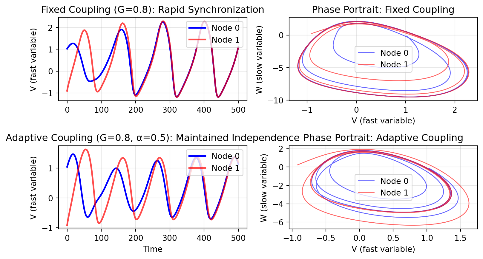
## Demonstrating Adaptive vs Fixed Coupling
We'll use two coupled oscillators with different initial conditions. Fixed coupling forces rapid synchronization, while adaptive coupling allows them to maintain more independent oscillations.
```{python}
from tvboptim.experimental.network_dynamics.dynamics.tvb import Generic2dOscillator

# Bidirectional coupling between two nodes
graph_osc = DenseGraph(jnp.array([[0.0, 1.0], [1.0, 0.0]]))

# Create oscillatory dynamics with different initial conditions per node
dynamics_fixed = Generic2dOscillator(
    a=2.0,    # Parameter controlling oscillation frequency
    b=-10.0,   # Damping
    c=0.0,
    d=0.02,
    tau=1.0,
    I=0.0,
    INITIAL_STATE=(1.0, 0.0)  # Node 0 starts here
)

dynamics_adaptive = Generic2dOscillator(
    a=2.0,
    b=-10.0,
    c=0.0,
    d=0.02,
    tau=1.0,
    I=0.0,
    INITIAL_STATE=(1.0, 0.0)
)

# Fixed coupling: strong constant gain
fixed_coupling = LinearCoupling(incoming_states='V', G=0.8)
network_fixed = Network(
    dynamics=dynamics_fixed,
    coupling={'instant': fixed_coupling},
    graph=graph_osc
)

# Adaptive coupling: same base gain but adapts
adaptive_coupling = AdaptiveGainCoupling(
    incoming_states='V',
    local_states='V',  # Need local state for adaptation
    G=0.8,
    alpha=0.9
)
network_adaptive = Network(
    dynamics=dynamics_adaptive,
    coupling={'instant': adaptive_coupling},
    graph=graph_osc
)

# Manually set different initial conditions for second node
initial_state_fixed = network_fixed.initial_state.at[:, 1].set(jnp.array([-1.0, 0.0]))
initial_state_adaptive = network_adaptive.initial_state.at[:, 1].set(jnp.array([-1.0, 0.0]))

# Update network history to use custom initial states
from tvboptim.experimental.network_dynamics.result import NativeSolution
network_fixed.update_history(NativeSolution(
    ts=jnp.array([0.0]),
    ys=initial_state_fixed[None, :, :],
    variable_names=tuple(network_fixed.dynamics.STATE_NAMES),
))
network_adaptive.update_history(NativeSolution(
    ts=jnp.array([0.0]),
    ys=initial_state_adaptive[None, :, :],
    variable_names=tuple(network_adaptive.dynamics.STATE_NAMES),
))

# Simulate both
result_fixed = solve(
    network_fixed, Euler(),
    t0=0.0, t1=500.0, dt=1.0
)

result_adaptive = solve(
    network_adaptive, Euler(),
    t0=0.0, t1=500.0, dt=1.0
)

print(f"Simulation complete: {len(result_fixed.ts)} time steps")
```
```{python}
#| code-fold: true
#| code-summary: "Visualization"
fig, axes = plt.subplots(2, 2, figsize=(8.1, 4.63))

# Time series - Fixed coupling
axes[0, 0].plot(result_fixed.ts, result_fixed.ys[:, 0, 0], 'b-', label='Node 0', linewidth=2)
axes[0, 0].plot(result_fixed.ts, result_fixed.ys[:, 0, 1], 'r-', label='Node 1', linewidth=2, alpha=0.7)
axes[0, 0].set_ylabel('V (fast variable)')
axes[0, 0].set_title('Fixed Coupling (G=0.8): Rapid Synchronization')
axes[0, 0].legend(loc='upper right')
axes[0, 0].grid(True, alpha=0.3)
# axes[0, 0].set_xlim(0, 100)

# Time series - Adaptive coupling
axes[1, 0].plot(result_adaptive.ts, result_adaptive.ys[:, 0, 0], 'b-', label='Node 0', linewidth=2)
axes[1, 0].plot(result_adaptive.ts, result_adaptive.ys[:, 0, 1], 'r-', label='Node 1', linewidth=2, alpha=0.7)
axes[1, 0].set_xlabel('Time')
axes[1, 0].set_ylabel('V (fast variable)')
axes[1, 0].set_title('Adaptive Coupling (G=0.8, α=0.5): Maintained Independence')
axes[1, 0].legend(loc='upper right')
axes[1, 0].grid(True, alpha=0.3)
# axes[1, 0].set_xlim(0, 100)

# Phase portraits - Fixed coupling
axes[0, 1].plot(result_fixed.ys[:, 0, 0], result_fixed.ys[:, 1, 0],
                'b-', linewidth=1, alpha=0.6, label='Node 0')
axes[0, 1].plot(result_fixed.ys[:, 0, 1], result_fixed.ys[:, 1, 1],
                'r-', linewidth=1, alpha=0.6, label='Node 1')
axes[0, 1].set_xlabel('V (fast variable)')
axes[0, 1].set_ylabel('W (slow variable)')
axes[0, 1].set_title('Phase Portrait: Fixed Coupling')
axes[0, 1].legend()
axes[0, 1].grid(True, alpha=0.3)

# Phase portraits - Adaptive coupling
axes[1, 1].plot(result_adaptive.ys[:, 0, 0], result_adaptive.ys[:, 1, 0],
                'b-', linewidth=1, alpha=0.6, label='Node 0')
axes[1, 1].plot(result_adaptive.ys[:, 0, 1], result_adaptive.ys[:, 1, 1],
                'r-', linewidth=1, alpha=0.6, label='Node 1')
axes[1, 1].set_xlabel('V (fast variable)')
axes[1, 1].set_ylabel('W (slow variable)')
axes[1, 1].set_title('Phase Portrait: Adaptive Coupling')
axes[1, 1].legend()
axes[1, 1].grid(True, alpha=0.3)

plt.tight_layout()
plt.show()
```
The key difference:
- **Fixed coupling**: Nodes quickly synchronize and oscillate in phase (overlapping trajectories)
- **Adaptive coupling**: Nodes maintain more independent oscillations with persistent phase differences
When oscillation amplitude increases, adaptive coupling reduces its strength, preventing complete synchronization. This demonstrates how `local_states` in `post()` enables state-dependent coupling mechanisms that can maintain network diversity despite strong structural connectivity.
# Delays
Brain networks exhibit transmission delays due to finite axonal conduction speeds. The `DelayedCoupling` base class handles delayed interactions automatically.
## Delay Computation
Delays are computed from tract lengths and conduction speed:
$$
\tau_{ij} = \frac{\text{length}_{ij}}{\text{speed}}
$$
The default conduction speed is **3 m/s** (typical for unmyelinated axons). Tract lengths are stored in the graph's delay matrix.
## Implementation Details
Delayed coupling maintains a **history buffer** - a circular buffer storing past states. During `compute()`, the appropriate delayed states are extracted based on connection-specific delays.
**Computational cost**: Delayed coupling requires more memory access for indexing into the history buffer at different time offsets per connection. This is more expensive than instantaneous coupling but essential for biological realism.
## Example
```{python}
from tvboptim.experimental.network_dynamics.coupling import DelayedLinearCoupling
from tvboptim.experimental.network_dynamics.graph import DenseDelayGraph
from tvboptim.experimental.network_dynamics.dynamics import Lorenz

# Create graph with delays (convert tract lengths to delays at 3 m/s)
weights_small = jnp.array([[0.0, 1.0], [1.0, 0.0]])
lengths_small = jnp.array([[0.0, 30.0], [30.0, 0.0]])  # 30 mm tract length
delays_small = lengths_small / 3.0

graph_delayed = DenseDelayGraph(weights_small, delays_small)

# Delayed coupling
delayed_coupling = DelayedLinearCoupling(incoming_states='x', G=0.5)

# Create network
network_delayed = Network(
    dynamics=Lorenz(),
    coupling=delayed_coupling,
    graph=graph_delayed
)

print(f"Tract length: {lengths_small[0, 1]} mm")
print(f"Conduction speed: 3 m/s (default)")
print(f"Delay: {lengths_small[0, 1] / 3:.1f} ms")
```
Delayed coupling requires `DelayGraph` (or `SparseDelayGraph`) which stores both weights and delays. See the [Graph](graph.qmd) section for details on delay graph construction.
# Multiple Couplings
Networks can have multiple coupling mechanisms simultaneously. Dynamics models declare which coupling inputs they expect via `COUPLING_INPUTS`:
```python
class MyDynamics(AbstractDynamics):
    COUPLING_INPUTS = {
        'instant': 1,   # Expects 1D instantaneous coupling
        'delayed': 1    # Expects 1D delayed coupling
    }

    def dynamics(self, t, state, params, coupling, external):
        c_instant = coupling.instant[0]
        c_delayed = coupling.delayed[0]
        # Use both in dynamics
        ...
```
When creating a network, provide couplings as a named dictionary:
```python
network = Network(
    dynamics=dynamics,
    coupling={
        'instant': LinearCoupling(incoming_states='S', G=1.0),
        'delayed': DelayedLinearCoupling(incoming_states='S', G=0.5)
    },
    graph=graph  # Must be DelayGraph for delayed coupling
)
```
**Key behavior**: If a dynamics model declares coupling inputs that are not provided, those inputs are **automatically filled with zeros**. This allows flexible configurations:
```python
# Model declares both instant and delayed, but only provide instant
network = Network(
    dynamics=dynamics,
    coupling={'instant': coupling_instant},  # 'delayed' will be zeros
    graph=graph
)
```
This zero-filling enables gradual model building and testing without requiring all coupling types upfront.
# Summary
See the [API Reference](../reference/index.qmd) for complete parameter descriptions and available coupling types.
Coupling enables inter-region communication in brain networks:
- **Lifecycle**: Three-phase pattern (`prepare` → `compute` → `update_state`) mirrors simulation flow
- **TVB pattern**: Most couplings use `pre()` → weighted sum → `post()` pattern; typically only `post()` needs implementation
- **Performance**: Vectorized mode (2D) faster for dense graphs; per-edge mode (3D) more flexible
- **Delays**: Computed from tract lengths and conduction speed; managed automatically via history buffers with increased computational cost
- **Multiple couplings**: Named dictionary with automatic zero-filling for missing inputs
- **Custom couplings**: Subclass `InstantaneousCoupling` or `DelayedCoupling` and override `pre()`/`post()`
Coupling integrates with [Dynamics](dynamics.qmd) through named inputs and with [Graph](graph.qmd) through connectivity structure. Together they define collective network behavior.